Ladder Logic Slides \[ \hat{H} = \frac{\hat{p}^2}{2m} + \frac{1}{2}m\omega^2\hat{x}^2 \]
\[ [\hat{x}, \hat{p}] = i\hbar \]
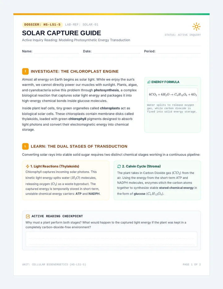
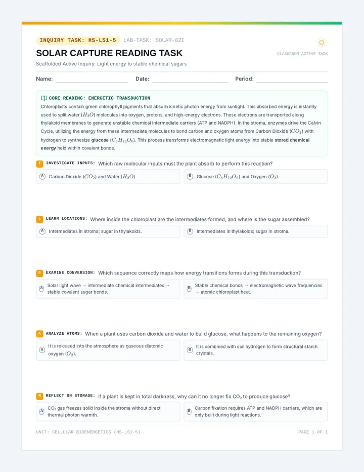
Ladder Logic
Canonical Quantization of the Harmonic Oscillator
Statistical & Quantum Mechanics Sequence
The Starting Point
01 // Hamiltonian
In classical mechanics, the harmonic oscillator Hamiltonian is a quadratic form:
\[ H = \frac{p^2}{2m} + \frac{1}{2}m\omega^2 x^2 \]
To quantize this system, we promote variables to operators:
\( x \rightarrow \hat{x} \)
\( p \rightarrow \hat{p} \)
Commutation: \( [\hat{x}, \hat{p}] = i\hbar \)
The Goal
We want to find the eigenvalues \( E_n \) and eigenstates \( |n\rangle \) such that:
\[ \hat{H}|n\rangle = E_n|n\rangle \]
Instead of solving the Schrodinger differential equation, we will use operator algebra.
Factoring the Hamiltonian
02 // Ladder Operators
We define dimensionless operators \( \hat{a} \) and \( \hat{a}^\dagger \):
\[ \hat{a} = \sqrt{\frac{m\omega}{2\hbar}} \left( \hat{x} + \frac{i\hat{p}}{m\omega} \right) \]
\[ \hat{a}^\dagger = \sqrt{\frac{m\omega}{2\hbar}} \left( \hat{x} - \frac{i\hat{p}}{m\omega} \right) \]
Commutation Relation:
\[ [\hat{a}, \hat{a}^\dagger] = 1 \]
Why do this?
The Hamiltonian can now be written in a remarkably simple form:
\[ \hat{H} = \hbar\omega \left( \hat{a}^\dagger \hat{a} + \frac{1}{2} \right) \]
We define the Number Operator: \[ \hat{N} = \hat{a}^\dagger \hat{a} \]
Climbing the Energy Levels
03 // Raising & Lowering
Annihilation (\( \hat{a} \))
Lowers the energy of a state by one quantum \( \hbar\omega \).
\[ \hat{a} |n\rangle = \sqrt{n} |n-1\rangle \]
Creation (\( \hat{a}^\dagger \))
Raises the energy of a state by one quantum \( \hbar\omega \).
\[ \hat{a}^\dagger |n\rangle = \sqrt{n+1} |n+1\rangle \]
Energy Spectrum: \[ E_n = \hbar\omega \left( n + \frac{1}{2} \right) \]
Where \( n = 0, 1, 2, \dots \)
Zero-Point Energy
04 // Ground State
The "ladder" must have a bottom. If it didn't, energy could be lowered to \( -\infty \), which is unphysical.
Defining the Ground State:
\[ \hat{a} |0\rangle = 0 \]
Applying the Hamiltonian to the ground state reveals the Zero-Point Energy.
\[ E_0 = \frac{1}{2}\hbar\omega \]
n=0 (Ground)
Even at absolute zero, the quantum oscillator possesses non-zero energy.
Why It Matters
05 // Conclusion
Algebra over Calculus
We derived the spectrum without solving a single differential equation.
The Template
Any system near a stable equilibrium can be modeled as a harmonic oscillator.
Field Bridge
These operators are the foundation for the "particles" of Quantum Field Theory.
Up Next: Coherent States & The Classical Limit
Operator Algebra Teacher Guide Operator Algebra Guide
Instructional Scaffolding: Canonical Quantization
Lesson 01 / Teacher Resource
Quantum Mechanics Sequence
Instructional Objectives
Conceptual Goals
Understand the shift from differential equations to operator algebra.
Appreciate the necessity of a lower bound on energy (the vacuum).
Visualize energy quantization as a "ladder" of discrete steps.
Technical Skills
Manipulation of the \([\hat{a}, \hat{a}^\dagger] = 1\) commutator.
Expressing \(\hat{x}\) and \(\hat{p}\) in terms of ladder operators.
Calculating expectation values using orthogonality.
Scaffolding the Derivation
1. The Factorization Trick
Start with the classical \( H = \frac{p^2}{2m} + \frac{1}{2}m\omega^2x^2 \). Point out it looks like \( A^2 + B^2 \), which factors to \((A-iB)(A+iB)\) in complex numbers. In quantum mechanics, because \([\hat{x}, \hat{p}] \neq 0\), the order matters.
Tip: Have students expand \( (\hat{x} - i\hat{p})(\hat{x} + i\hat{p}) \) to see the "extra" commutator term arise.
2. The Commutator Lemma
The core of the ladder method is the identity \([\hat{H}, \hat{a}] = -\hbar\omega\hat{a}\). Prove this carefully. It demonstrates that if \(|n\rangle\) is an eigenstate, \(\hat{a}|n\rangle\) is also an eigenstate with energy \(E - \hbar\omega\).
Key Question: "If we keep applying \(\hat{a}\), does the energy go to negative infinity?" Use this to motivate the definition of the ground state \(\hat{a}|0\rangle = 0\).
3. Normalization Factors
Students often forget why \(\hat{a}|n\rangle = \sqrt{n}|n-1\rangle\) instead of just \(|n-1\rangle\). Use the requirement that \(\langle n-1 | n-1 \rangle = 1\):
\[ \langle n | \hat{a}^\dagger \hat{a} | n \rangle = \langle n | \hat{N} | n \rangle = n \]
Common Misconceptions
"The ground state energy is zero." Clarify that \(\hat{a}|0\rangle = 0\) is the state vector being nullified, but the energy \(E_0 = \frac{1}{2}\hbar\omega\) is non-zero due to the uncertainty principle.
"Operators are numbers." Remind students that \(\hat{a}\hat{a}^\dagger \neq \hat{a}^\dagger\hat{a}\). This is the single most common source of algebraic error in the course.
Discussion Prompts
Why is the harmonic oscillator potential so ubiquitous in physics?
Answer: Any smooth potential looks quadratic near its minimum (Taylor expansion).
Ladder Logic Worksheet Ladder Logic Problem Set
Statistical & Quantum Mechanics of Oscillators
Name:
Date:
1
The Fundamental Commutator
Given the definitions of the annihilation and creation operators: \[ \hat{a} = \sqrt{\frac{m\omega}{2\hbar}} \left( \hat{x} + \frac{i\hat{p}}{m\omega} \right) \quad \text{and} \quad \hat{a}^\dagger = \sqrt{\frac{m\omega}{2\hbar}} \left( \hat{x} - \frac{i\hat{p}}{m\omega} \right) \] Prove that \( [\hat{a}, \hat{a}^\dagger] = 1 \) using the canonical commutation relation \( [\hat{x}, \hat{p}] = i\hbar \). Show every algebraic step.
2
Expectation Values in the n-th State
Using the fact that \( \hat{x} = \sqrt{\frac{\hbar}{2m\omega}}(\hat{a} + \hat{a}^\dagger) \), calculate the expectation value of the position squared, \( \langle n | \hat{x}^2 | n \rangle \), for an arbitrary eigenstate \( |n\rangle \).
3
Equipartition of Quantum Energy
Based on your result in Problem 2, find the expectation value of the potential energy \( \langle V \rangle = \frac{1}{2}m\omega^2 \langle \hat{x}^2 \rangle \). Show that it is equal to exactly half of the total energy \( E_n \). What does this imply about the kinetic energy \( \langle T \rangle \)?
Physical Insight
The result \( \langle T \rangle = \langle V \rangle = \frac{1}{2} E_n \) is a specific case of the Quantum Virial Theorem for quadratic potentials. Even in the quantum regime, the symmetry between kinetic and potential energy in a harmonic oscillator is preserved.
Coherent States Slides Coherent States
The Quantum-Classical Bridge
Lesson 02 // Dynamics & Uncertainty
Eigenstates of the Annihilation Operator
01 // Definition
Energy eigenstates \( |n\rangle \) are stationary. They don't "oscillate" in a classical sense.
A Coherent State \( |\alpha\rangle \) is an eigenstate of the annihilation operator:
\[ \hat{a} |\alpha\rangle = \alpha |\alpha\rangle \]
where \( \alpha \) is a complex number representing the amplitude and phase.
Expansion in Energy Basis
The coherent state is a superposition of all infinite energy levels:
\[ |\alpha\rangle = e^{-|\alpha|^2/2} \sum_{n=0}^{\infty} \frac{\alpha^n}{\sqrt{n!}} |n\rangle \]
The distribution of energy levels follows Poisson Statistics .
Minimum Uncertainty States
02 // Uncertainty
Coherent states are unique because they "saturate" the Heisenberg Uncertainty Principle and maintain it over time.
\[ \Delta x \Delta p = \frac{\hbar}{2} \]
Unlike generic wave packets, coherent states do not spread as they evolve.
p
x
In phase space, a coherent state is a circle of constant area that orbits the origin.
Classical Trajectories
03 // Dynamics
The time evolution of the parameter \( \alpha \) is simple phase rotation:
\[ \alpha(t) = \alpha(0) e^{-i\omega t} \]
This leads to the expectation values:
\( \langle \hat{x} \rangle_t = x_{cl}(t) \)
\( \langle \hat{p} \rangle_t = p_{cl}(t) \)
The Classical Limit
As \( |\alpha| \rightarrow \infty \), the relative fluctuations \( \Delta x / \langle x \rangle \) vanish.
Large amplitude coherent states are the quantum description of a macroscopic mass on a spring.
Key Takeaways
04 // Conclusion
Precision
They provide the lowest possible noise allowed by quantum mechanics.
Stability
The wavepacket maintains its shape throughout its entire motion.
Applications
Fundamental for Quantum Optics and Laser physics.
Next Lesson: The Statistical Thermodynamics of Oscillators
Classical Limit Teacher Guide Classical Limit Guide
Instructional Scaffolding: Coherent States
Lesson 02 / Teacher Resource
Quantum Mechanics Sequence
Core Conceptual Pillars
The Definition
Defining $|\alpha\rangle$ as an eigenstate of $\hat{a}$ rather than $\hat{H}$. This is the "trick" to finding states that aren't stationary.
Phase Space
Visualizing the state as a "fuzzy ball" of probability orbiting the origin without changing size or shape.
Correspondence
Showing how quantum fluctuations become negligible as the amplitude $\alpha$ becomes large.
The Displacement Operator Approach
While $|\alpha\rangle$ is defined by $\hat{a}$, students often struggle with where it "comes from." Use the Displacement Operator to motivate it physically:
\[ \hat{D}(\alpha) = \exp(\alpha\hat{a}^\dagger - \alpha^*\hat{a}) \]
Explain that $\hat{D}(\alpha)$ "kicks" the ground state from the origin to a location $\alpha$ in phase space. The coherent state is simply: \( |\alpha\rangle = \hat{D}(\alpha) |0\rangle \)
Teaching Tip: Connect this to the "Squeezed States" discussion if time permits. A squeezed state is one where $\Delta x \neq \Delta p$, but their product still equals $\hbar/2$. A coherent state is the special case of equal uncertainty.
Handling the Classical Paradox
Students often ask: "If particles are wavefunctions, why don't I see my car spreading out in the parking lot?"
Use coherent states to answer this. Calculate the fractional uncertainty for a macroscopic mass (e.g., 1kg) on a spring (1Hz). Show that $\Delta x / x$ is on the order of $10^{-17}$, far below the threshold of human measurement. The "car" is indeed spreading, but the rate is so minuscule that it's effectively rigid.
Problem Solving Guidance
Technique: Baker-Campbell-Hausdorff (BCH)
Students will encounter terms like $e^{\hat{A}+\hat{B}}$ when dealing with displacement operators. Remind them of the special case for commutators that are c-numbers:
\[ e^{\hat{A}}e^{\hat{B}} = e^{\hat{A}+\hat{B}}e^{\frac{1}{2}[\hat{A}, \hat{B}]} \]
This identity is critical for proving that coherent states are normalized.
Minimum Uncertainty Handout Minimum Uncertainty Exploration
Lesson 02: Dynamics of the Coherent State
Name:
1
The Overlap Integral
Unlike energy eigenstates \( |n\rangle \), coherent states are not orthogonal. Calculate the overlap between two coherent states \( |\alpha\rangle \) and \( |\beta\rangle \): \[ \langle \beta | \alpha \rangle = e^{-\frac{1}{2}(|\alpha|^2 + |\beta|^2) + \beta^*\alpha} \] What happens to the overlap as the distance between the states in phase space, \( |\alpha - \beta| \), increases?
2
Uncertainty Calculation
For a coherent state \( |\alpha\rangle \), we know \( \langle \hat{a} \rangle = \alpha \). Using the relationship \( \hat{x} = \sqrt{\frac{\hbar}{2m\omega}}(\hat{a} + \hat{a}^\dagger) \), show that: \[ (\Delta x)^2 = \langle \hat{x}^2 \rangle - \langle \hat{x} \rangle^2 = \frac{\hbar}{2m\omega} \] Note that this value is independent of \( \alpha \). Repeat for \( (\Delta p)^2 \) and verify that the Heisenberg product is saturated.
3
Number Statistics
A coherent state \( |\alpha\rangle \) contains a variable number of energy quanta (photons). The probability of finding \( n \) quanta is given by \( P(n) = |\langle n | \alpha \rangle|^2 \).
a) Show that \( P(n) \) follows a Poisson Distribution : \( P(n) = \frac{\lambda^n e^{-\lambda}}{n!} \). What is \( \lambda \) in terms of \( \alpha \)?
b) Calculate the mean number of quanta \( \langle \hat{N} \rangle \).
Thinking Cap
Why does a laser (which produces coherent states) behave differently than a light bulb (which produces thermal states)? Consider the "noise" or "variance" in the photon number.
Partition Function Slides \[ Z = \sum e^{-\beta E_n} \]
Thermal Ensembles
Statistical Mechanics of the Oscillator
Lesson 03 // Partition Functions & Free Energy
Summing the States
01 // The Z-Function
For a quantum oscillator in thermal contact with a reservoir at temperature \( T \), the partition function is:
\[ Z = \sum_{n=0}^{\infty} e^{-\beta \hbar\omega(n + 1/2)} \]
where \( \beta = 1/k_B T \).
The Result
Evaluating the geometric series yields:
\[ Z = \frac{e^{-\beta\hbar\omega/2}}{1 - e^{-\beta\hbar\omega}} \]
This single function contains all thermodynamic information about the system.
The Internal Energy
02 // Energy & Heat
The average energy \( \langle E \rangle \) is derived from \( Z \):
\[ \langle E \rangle = \frac{\hbar\omega}{2} + \frac{\hbar\omega}{e^{\beta\hbar\omega} - 1} \]
Term 1: Zero-point energy (Quantum).
Term 2: Thermal excitation (Statistical).
Classical (kBT)
Quantum Spectrum
Energy
Temperature
At high temperatures, we recover the classical \( k_B T \) result.
Quantum Freeze-Out
03 // Thermodynamics
Why Equipartition Fails
In classical physics, every degree of freedom gets \( \frac{1}{2}k_B T \).
But if \( k_B T \ll \hbar\omega \), the thermal energy is not enough to excite the oscillator to the first level.
The oscillator is "frozen out" of the thermodynamics, contributing nothing to the heat capacity.
Ultraviolet Catastrophe
Quantum mechanics prevents high-frequency modes from sucking all the energy out of a system.
Planck's Insight
Energy quantization was the only way to resolve the infinite energy paradox of blackbody radiation.
Scale Up
04 // Moving Forward
We have solved for one oscillator.
What happens if we have \( 10^{23} \) of them?
Solids
Atomic lattice vibrations (Phonons).
Fields
Radiation modes in a cavity.
Next: Einstein and Debye Models of Solids
Statistical Mechanics Teacher Guide Statistical Mechanics Guide
Instructional Scaffolding: The Thermal Oscillator
Lesson 03 / Teacher Resource
Quantum Mechanics Sequence
The Mathematical Path
1. The Geometric Series
Remind students of the sum \(\sum_{n=0}^{\infty} r^n = \frac{1}{1-r}\) for \(|r| < 1\). In the partition function, \(r = e^{-\beta\hbar\omega}\). Since \(\beta, \hbar, \omega > 0\), the series always converges.
2. Logarithmic Derivatives
The link between statistics and thermodynamics is the identity: \[ \langle E \rangle = -\frac{\partial \ln Z}{\partial \beta} \] Scaffold the derivation by having students take the derivative of \(\ln(1-e^{-\beta\hbar\omega})\) using the chain rule.
3. The High-T Limit
Use the Taylor expansion \(e^x \approx 1 + x\) for small \(x\). In the high-temperature limit (\(\beta \rightarrow 0\)), the average energy becomes: \[ \langle E \rangle \approx \frac{\hbar\omega}{2} + \frac{\hbar\omega}{(1 + \beta\hbar\omega) - 1} = \frac{\hbar\omega}{2} + k_B T \] This recovers the classical Equipartition Theorem (minus the zero-point shift).
Key Discussion Points
The "Ultraviolet" Problem
Ask: "If classical mechanics were right, why wouldn't every atomic vibration at 1,000,000 Hz immediately suck all the heat out of the room?"
Answer: Because \(k_B T\) at room temperature is too small to overcome the \(\hbar\omega\) jump of high-frequency modes.
Entropy and Information
Discuss how entropy \(S = -\frac{\partial F}{\partial T}\) relates to the number of accessible states. At low \(T\), only the ground state is accessible, so \(S \rightarrow 0\), consistent with the Third Law.
Common Student Hurdles
Confusing \(\beta\) and \(T\): Many students will differentiate with respect to \(T\) and get bogged down in algebra. Encourage them to stay in "beta-space" for all derivatives and only convert back to \(T\) at the very end.
Zero-Point Energy in Thermo: Does \(E_0\) matter for \(C_V\)? No, because it's a constant. Does it matter for \(F\)? Yes. Clarify what "observable" quantities are affected by the shift.
Quantum Statistics Problems Thermal Oscillator Problems
Lesson 03: Partition Functions & Thermodynamics
Student Name:
1
Free Energy Derivation
Starting from the quantum partition function for a single harmonic oscillator: \[ Z = \frac{e^{-\beta\hbar\omega/2}}{1 - e^{-\beta\hbar\omega}} \] Calculate the Helmholtz Free Energy \( F = -k_B T \ln Z \). Write your answer in terms of \( \beta \) and then in terms of \( T \).
2
The Specific Heat
The internal energy is \( \langle E \rangle = \frac{\hbar\omega}{2} + \frac{\hbar\omega}{e^{\beta\hbar\omega}-1} \). Derive the Heat Capacity at constant volume, \( C_V = \left( \frac{\partial \langle E \rangle}{\partial T} \right)_V \). Show that \( C_V \) goes to zero exponentially as \( T \rightarrow 0 \).
3
The N-Oscillator System
Consider a system of \( N \) independent, identical quantum harmonic oscillators.
a) Write the total partition function \( Z_N \) in terms of the single-oscillator \( Z \).
b) Calculate the total average energy \( U = \langle E_{total} \rangle \).
c) If these oscillators represent atoms in a 3D crystal (where each atom has 3 degrees of freedom), how many total oscillators are there for \( N \) atoms?
Connection to Solids
In the next lesson, we will use this exact result to build the **Einstein Model** of heat capacity in solids. You have just derived the mathematical engine that drives solid-state thermodynamics.
Einstein Debye Slides Solid State Oscillators
The Einstein and Debye Models
Lesson 04 // Lattice Vibrations & Heat Capacity
Independent Oscillators
01 // Einstein Model (1907)
Einstein assumed every atom in a solid is an independent 3D harmonic oscillator.
Key Assumptions:
All atoms vibrate at the same frequency \(\omega_E\).
They do not interact with their neighbors.
\[ C_V = 3Nk_B \left( \frac{\hbar\omega_E}{k_B T} \right)^2 \frac{e^{\hbar\omega_E/k_B T}}{(e^{\hbar\omega_E/k_B T}-1)^2} \]
Success & Failure
Success: Correctly predicts that \( C_V \rightarrow 0 \) as \( T \rightarrow 0 \). (Solves the classical failure).
Failure: It goes to zero too fast (exponentially), whereas experiments show a \( T^3 \) power law.
Coupled Vibrations
02 // Debye Model (1912)
The "Phonon" approach
Instead of independent atoms, Debye modeled the solid as a continuous medium supporting sound waves.
Atoms are coupled; they move in waves.
Low-frequency waves (long wavelengths) are easy to excite.
High-frequency waves are limited by the atomic spacing (Debye cutoff).
Density of States
\[ g(\omega) \propto \omega^2 \]
More modes available at higher frequencies.
The Low-T Result
\[ C_V \propto T^3 \]
Matches experimental data perfectly.
The Mode Spectrum
03 // Comparison
Einstein
\( \omega_E \)
Delta function at one frequency.
vs
Debye
\( \omega_D \)
Quadratic distribution up to a cutoff.
Closing the Loop
04 // Conclusion
The Debye model treats vibrations as field excitations.
This is the birth of Second Quantization.
Discrete Atoms
Move together to form collective modes.
Quasiparticles
These modes behave exactly like independent harmonic oscillators.
Next Lesson: Field Theory — The Vacuum of Infinite Oscillators
Heat Capacity Guide Specific Heat Guide
Instructional Scaffolding: Lattice Models
Lesson 04 / Teacher Resource
Quantum Mechanics Sequence
The Modeling Shift
Einstein's Simplification
Einstein's genius was realizing that the discrete energy levels of an oscillator would "freeze out" at low $T$. However, he missed the collective nature of solids.
Focus: Use this to illustrate how a simple model can capture the qualitative physics while failing the quantitative details.
Debye's Sophistication
Debye realized that low-energy excitations in solids are long-wavelength sound waves (phonons), which have very low frequencies.
Focus: This is where you introduce the **Density of States** $g(\omega)$. It is the first time students see that not all frequencies are created equal.
Scaffolding the $T^3$ Law
The integral for total energy in the Debye model is:
\[ U = \int_0^{\omega_D} \frac{\hbar\omega}{e^{\beta\hbar\omega}-1} g(\omega) d\omega \]
Since $g(\omega) = A\omega^2$, we substitute $x = \beta\hbar\omega$. For low $T$, $\beta \rightarrow \infty$, so the limit of integration goes to infinity.
\[ U \propto T^4 \int_0^\infty \frac{x^3}{e^x-1} dx \implies C_V \propto T^3 \]
Note: The integral is a standard Zeta function form. Don't let students get lost in the integration; focus on the temperature scaling.
Discussion: What is a Phonon?
A phonon is a **quasiparticle**. It is not a piece of matter, but a "quantized packet of sound."
Ask students: "Does a phonon obey the same ladder operator math as our mass-on-a-spring?"
Answer: Yes! The Hamiltonian for the lattice can be transformed into a sum of independent harmonic oscillators in $k$-space. This is the ultimate "power move" of physics: turning a complex, coupled problem into many simple ones.
Feature Einstein Debye Nature of Osc. Independent Atoms Collective Modes (Waves) Freq. Spectrum Single frequency $\omega_E$ Continuous up to $\omega_D$ Low-T Limit Exponentially zero Power law $T^3$
Lattice Vibration Worksheet Lattice Vibration Worksheet
Lesson 04: From Atoms to Phonons
Name:
1
The Einstein Scale
The Einstein temperature is defined as \( \Theta_E = \hbar\omega_E / k_B \). For Diamond, \( \Theta_E \approx 1320 \) K. For Lead, \( \Theta_E \approx 70 \) K.
a) Which material is "more quantum" at room temperature (300 K)? Explain why.
b) Calculate the Heat Capacity \( C_V \) (per mole) for Diamond at 300 K using the Einstein formula.
2
Counting Modes
In the Debye model, the density of states is \( g(\omega) = \frac{3V\omega^2}{2\pi^2 v^3} \), where \( v \) is the speed of sound. The Debye frequency \( \omega_D \) is found by integrating \( g(\omega) \) and setting the result equal to the total degrees of freedom, \( 3N \).
Derive the expression for \( \omega_D \) in terms of the atomic density \( N/V \) and sound speed \( v \).
3
Comparison to Reality
Below is a conceptual plot of \( C_V \) vs \( T \). Sketch the predictions for the Classical model (Dulong-Petit), the Einstein model, and the Debye model. Label the \( T^3 \) region and the high-T limit.
T (Kelvin)
Cv (Heat Capacity)
Thinking Challenge: Why does the speed of sound \( v \) appear in the Debye model but not in the Einstein model? What does this tell us about the relationship between thermodynamics and acoustics?
Field Quantization Slides Field Theory
The Universe as an Ensemble of Oscillators
Lesson 05 // Second Quantization & The Vacuum
The Continuum Limit
01 // Transition
In Lesson 4, we saw that a lattice of atoms becomes a collection of normal modes.
A continuous field (like the electromagnetic field) is just the limit where the number of oscillators goes to infinity.
The Mapping
Spatial Mode \( k \) \( \rightarrow \) One Oscillator
Energy Level \( n \) \( \rightarrow \) Number of Particles
Every field is a sum over an infinite number of independent harmonic oscillators.
Creation & Annihilation
02 // Formalism
We promote the field amplitudes to operators \( \hat{a}_k \) and \( \hat{a}_k^\dagger \).
The Hamiltonian of the Universe:
\[ \hat{H}_{field} = \sum_k \hbar\omega_k \left( \hat{a}_k^\dagger \hat{a}_k + \frac{1}{2} \right) \]
Each mode \( k \) behaves exactly like the quantum oscillator we studied in Lesson 1.
Particles as Excitations
A "particle" is no longer a tiny ball. A particle is a unit of excitation in a field oscillator.
One photon = The \( n=1 \) state of the EM mode at frequency \( \omega \).
The Zero-Point Crisis
03 // The Vacuum
The term \( \frac{1}{2}\hbar\omega_k \) exists for every mode \( k \).
The Divergence:
\[ E_{vac} = \sum_k \frac{1}{2}\hbar\omega_k \rightarrow \infty \]
This suggests that even "empty" space contains an infinite amount of energy.
Physical Effects
Casimir Effect: Plates being pushed together by vacuum fluctuations.
Lamb Shift: Small energy shifts in atoms due to vacuum interaction.
Cosmology: The Dark Energy problem (the worst prediction in physics).
The Universal Model
04 // Finale
"The harmonic oscillator is the most important system in physics because, to a first approximation, everything is a harmonic oscillator."
Atomic Bonds
Solid State
Light / Optics
Quantum Fields
End of Sequence // Statistical & Quantum Mechanics
Vacuum Energy Guide Vacuum Energy Guide
Instructional Scaffolding: Field Quantization
Lesson 05 / Teacher Resource
Quantum Mechanics Sequence
The Continuum Jump
The most difficult conceptual leap for students in this lesson is the transition from particles (discrete objects) to fields (continuous distributions). Use the following scaffolding:
The 1D String Analogy
Start with a string of $N$ masses and $N+1$ springs. Derive the normal modes. Show that as $N \rightarrow \infty$, the discrete masses become a continuous density $\mu$, and the normal modes become a Fourier series.
The Energy Mapping
Explain that in "First Quantization," the oscillator is a particle moving in a potential. In "Second Quantization," the field itself is the oscillator, and the "particles" are the energy levels $n$ of that oscillator.
Handling the Infinite Sum
The Problem:
\[ E_{total} = \sum_k \left( n_k + \frac{1}{2} \right) \hbar\omega_k \]
When students see this, they will point out that even if all $n_k = 0$, the energy is infinite. This is the **Zero-Point Energy** of the vacuum.
Pedagogical Pivot:
Explain that in most physics, we only care about energy differences . We can "re-normalize" the vacuum by subtracting the infinite constant. However, in General Relativity, absolute energy matters (gravity sees it). This remains the greatest unsolved problem in modern physics.
Final Discussion Prompts
If the vacuum has energy, why don't we feel it?
Answer: Because it's uniform. Much like fish in water don't "feel" the pressure unless it changes, we only see the vacuum's effect when we introduce boundaries (Casimir Effect) or fluctuations.
Why is the harmonic oscillator the "fundamental block"?
Answer: Because any field, when linearized, is a collection of non-interacting modes. And any non-interacting mode obeys the same quadratic energy structure as a spring.
Statistical & Quantum Mechanics Sequence Complete
Normal Mode Handout Normal Mode Mapping
Lesson 05: The Field as an Oscillator Collection
Name:
1
The Mass-Spring Chain
Consider a chain of \( N \) identical masses \( m \) connected by springs \( \kappa \). The displacement of the \( j \)-th mass is \( q_j \). The equations of motion are coupled: \[ m\ddot{q}_j = -\kappa(2q_j - q_{j-1} - q_{j+1}) \] By transforming to Normal Coordinates \( Q_k = \sum e^{ikja} q_j \), we can decouple these into \( N \) independent harmonic oscillators.
Calculate the dispersion relation \( \omega(k) \) for this chain. Show that for small \( k \), it looks like sound: \( \omega = vk \).
2
Field Hamiltonian
A continuous scalar field \( \phi(x,t) \) can be expanded in terms of ladder operators: \[ \hat{\phi}(x) = \sum_k \sqrt{\frac{\hbar}{2\omega_k V}} \left( \hat{a}_k e^{ikx} + \hat{a}_k^\dagger e^{-ikx} \right) \] Given the field Hamiltonian \( \hat{H} = \frac{1}{2} \int [ \dot{\phi}^2 + (\nabla\phi)^2 ] dV \), substitute the expansion and show that it simplifies to: \[ \hat{H} = \sum_k \hbar\omega_k (\hat{a}_k^\dagger \hat{a}_k + 1/2) \]
3
Vacuum Pressure
The Casimir effect arises because a boundary (like two plates) limits the number of allowed modes \( k \).
a) If two plates are at distance \( L \), the allowed modes are \( k_n = n\pi/L \). Write the sum for the total zero-point energy between the plates.
b) Qualitatively, why does this energy change as the plates move closer together? What does this imply about the force (pressure) between the plates?
Synthesis
Over this sequence, we moved from one mass on a spring to the infinite collection of oscillators that define the vacuum of space. You are now prepared for Quantum Field Theory.