Wave Birth Slides Wave Birth
Hertzian Dipoles & Wave Generation
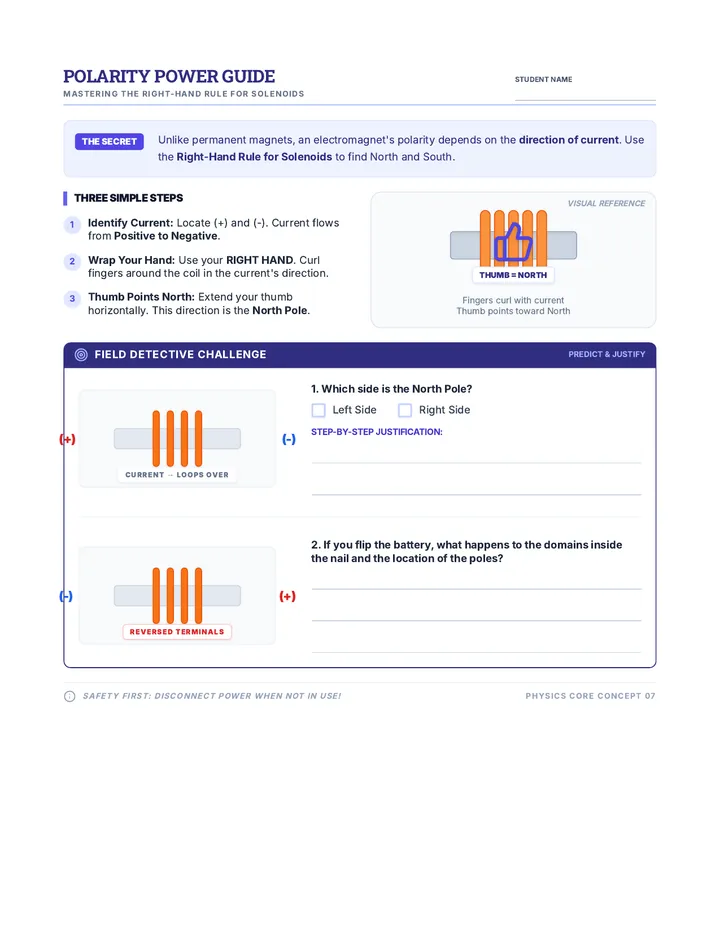
The Core Mystery
How do waves "escape" the wire?
Consider a simple alternating current in a rod. We know it creates a local magnetic field and electric field.
But at what point does this field stop being a static "shroud" around the metal and become a traveling wave that detaches forever?
Current (I) ↔ Fields (E, B)
The Hertzian Dipole Model
Definition
An infinitesimal segment of current \( dl \) with a uniform current distribution \( I(t) = I_0 \cos(\omega t) \).
Conditions
\( dl \ll \lambda \) (Small compared to wavelength)
Oscillating dipole moment \( p(t) = q(t) dl \)
Near Field vs. Far Field
Spatial Duality
Near Field (Reactive)
Dominated by \( 1/r^2 \) and \( 1/r^3 \) terms. Energy oscillates back and forth between the antenna and space.

\[ E \propto \frac{1}{r^3}, \quad B \propto \frac{1}{r^2} \]
No real power loss to space.
Far Field (Radiative)
Dominated by \( 1/r \) terms. Energy detaches and propagates outward as a self-sustaining wave.


\[ E \propto \frac{1}{r}, \quad B \propto \frac{1}{r} \]
The birth of the EM wave.
Radiation Resistance
To the circuit, the act of "throwing" energy into space looks exactly like loss.
\[ P_{rad} = I_{rms}^2 R_{rad} \]
Where \( R_{rad} = 80\pi^2 (dl/\lambda)^2 \) for a short dipole.
The higher the frequency (shorter \( \lambda \)), the more efficiently we can couple energy to space.
Key Takeaways
1
Oscillating charges create both induction and radiation fields.
2
The far-field detaches as \( 1/r \) components dominate.
3
Antenna size relative to wavelength determines radiation efficiency.
Next Lesson: Antenna Radiation Patterns
Wave Birth Worksheet Wave Birth Worksheet
Hertzian Dipoles & Wave Generation
Name:
Date:
Objective: To mathematically analyze the components of an electromagnetic field generated by a short dipole antenna and distinguish between the induction and radiation zones.
01 Analyzing the E-Field Components
The electric field \( E_\theta \) of a Hertzian dipole in spherical coordinates is given by: \[ E_\theta = \frac{p_0 k^3}{4\pi\epsilon_0} \sin\theta \left[ \frac{j}{kr} + \frac{1}{(kr)^2} - \frac{j}{(kr)^3} \right] e^{j(\omega t - kr)} \]
A. Identify which term in the brackets represents the "Radiation Field" and explain why its dependence on distance \( r \) is critical for long-range communication.
B. Define the "Fraunhofer Distance" (Far-field boundary). At what value of \( kr \) do the magnitude of the \( 1/r \) and \( 1/r^2 \) terms become equal?
02 The Efficiency of the Dipole
A short dipole has a length \( dl = 0.05\lambda \). The current amplitude is \( I_0 = 2 \, \text{A} \).
A. Calculate the radiation resistance \( R_{rad} \) using the formula \( R_{rad} = 80\pi^2 (dl/\lambda)^2 \).
B. Calculate the total power radiated by this antenna. Recall \( P_{rad} = \frac{1}{2} I_0^2 R_{rad} \).
C. If the antenna has an ohmic (heat) resistance of \( 0.5 \, \Omega \), calculate the radiation efficiency \( \eta = \frac{R_{rad}}{R_{rad} + R_{ohmic}} \).
03 Field Visualization
In the space below, sketch the electric field lines around a vertical dipole at a single moment in time. Indicate the "detachment" point where loops of field lines begin to move away from the source.
Sketch Area: Electric Field Lines
RF Engineering Sequence • Lesson 1 • Physics of Wave Generation
Wave Birth Teacher Guide Teacher Guide Sequence: Wave Runners RF
Wave Birth Physics
Hertzian Dipoles & Wave Generation Instructional Framework
Instructional Goal
This lesson bridges the gap between static/low-frequency electromagnetics and radiative wave physics. Students often struggle with the conceptual "detachment" of the field. The goal is to show that radiation is not a separate phenomenon but a consequence of the phase lag and distance dependency of Maxwell's equations.
Key Concepts to Emphasize:
Induction Field: Energy stored in the near-zone; returns to the source every half-cycle.
Radiation Field: The \( 1/r \) term that carries power to infinity.
Phase Difference: The 90-degree phase difference in the near-field (reactive) vs. the in-phase E and H in the far-field (resistive).
Pacing Guide
00-10 min
Hook & Field Mystery
10-30 min
Dipole Math & Components
30-50 min
Near vs. Far Field Lab/Worksheet
50-60 min
Discussion: Why size matters?
Discussion Prompts
The "Detachment" Paradox
"If we stop the current in the antenna instantly, what happens to the waves that have already reached the far-field? Why can't they come back?"
The 50/60Hz Problem
"Power lines carry high alternating current. Why don't they act as giant antennas and radiate all our power into space?"
Common Student Misconceptions
"Radiation is different from Fields": Students often think of radiation as "stuff" being shot out. Clarify that it is the spatial-temporal rearrangement of the same field lines.
"Near-field is always small": At low frequencies (like 60Hz), the near-field extends for thousands of kilometers. At high frequencies (GHz), it is mere millimeters.
Worksheet Quick-Key
// Question 1B: Transition Point
Transition happens when kr = 1. Distance r = λ / 2π.
// Question 2A: Radiation Resistance
R_rad = 80 * π^2 * (0.05)^2 ≈ 1.97 Ω.
// Question 2C: Efficiency
η = 1.97 / (1.97 + 0.5) ≈ 79.7%.
Radiation Reach Slides Radiation Reach
Antenna Characteristics & Radiation Patterns
Form Follows Function
Why aren't all antennas just straight wires?
Isotropic
Ideally sends energy in every direction. Great for phones that move.
Directional
Beams energy in one direction. High "Gain," longer reach.
Array
Multiple elements working together to "shape" the beam.
The Efficiency Metrics
Directivity (D)
The ratio of radiation intensity in a given direction to the average radiation intensity. It's a measure of "focus."
Gain (G)
Directivity multiplied by efficiency (\( \eta \)). It accounts for both focus and internal ohmic losses.
G = ηD
"Gain doesn't create energy; it just steals it from other directions to strengthen the main beam."
Visualizing Radiation Patterns
Main Lobe
Back Lobe
Key Pattern Landmarks:
Half-Power Beamwidth (HPBW):
The angular width where power drops by 3dB.
Side Lobes:
Unwanted radiation in unintended directions.
Front-to-Back Ratio:
How much better it looks forward than backward.
The Handshake
If the Antenna Impedance doesn't match the Transmission Line, energy bounces back.
The Consequence
VSWR
Voltage Standing Wave Ratio. High VSWR = Danger to the transmitter.
Ideal Match
Zline = 50 Ω Zant = 50 Ω
Maximum Power Transfer
Lessons Summary
Antennas concentrate energy; they don't amplify it. High gain means high focus.
Patterns are 3D, but we analyze them via 2D polar slices (Azimuth & Elevation).
HPBW determines the precision needed for antenna pointing.
Matching ensures the power actually leaves the transmitter.
Radiation Reach Activity Sheet Radiation Reach Activity
Pattern Interpretation & Design Optimization
Student Identifier
Part 01
Interpreting the Polar Plot
0° 180°
Normalized Radiation Pattern (dB)
1. Estimate the Half-Power Beamwidth (HPBW)
Identify the angle between the -3dB points on the main lobe.
2. Identify the Front-to-Back Ratio (F/B)
Calculate the dB difference between peak of main lobe and peak of back lobe.
3. Practical Application
Would this antenna be suitable for a fixed point-to-point microwave link? Why or why not?
Part 02
Gain Metrics
Calculated Directivity
12.5 dBi
Internal Loss
-0.8 dB
Input Power
100 mW
A. Calculate the total Antenna Gain in dBi.
B. Calculate the EIRP (Effective Isotropic Radiated Power) in dBm.
C. Conceptual Design: How would increasing the number of elements in a Yagi-Uda array affect the HPBW and the Gain?
Part 03
Impedance Matching Challenge
A transmitter with a 50 Ω output is connected to an antenna with an input impedance of 75 Ω.
Reflectance Coefficient (Γ)
\[ \Gamma = \frac{Z_L - Z_0}{Z_L + Z_0} \]
Calculate Value
Resulting VSWR
\[ VSWR = \frac{1+|\Gamma|}{1-|\Gamma|} \]
Identify the percentage of incident power reflected back to the transmitter.
RF Engineering Course Lesson 2: Antenna Reach & Patterns Page 01 of 01
Signal Morphing Slides Signal Morphing
Modulation Techniques & Spectrum
The Carrier Paradox
A pure sine wave carries exactly zero information.
To send data, we must perturb the wave. We change one of three variables over time:
A Amplitude
f Frequency
φ Phase
Information = Change = Bandwidth
Amplitude Modulation (AM)
The instantaneous amplitude of the carrier wave follows the amplitude of the baseband (audio) signal.
\[ s(t) = [A_c + m(t)] \cos(2\pi f_c t) \]
Where \( m(t) \) is the information signal.
Time Domain Visualization
"The Envelope carries the message."
Frequency Modulation (FM)
Constant Amplitude, Variable Speed
Immune to static (amplitude noise), but consumes more bandwidth.
The instantaneous frequency of the carrier is shifted from its center frequency by an amount proportional to the signal voltage.
Key Advantage
Better Signal-to-Noise Ratio (SNR) and high fidelity, but requires a wider "chunk" of the spectrum.
The Frequency Domain
Sideband Anatomy
Multiplying signals in the time domain leads to convolution in the frequency domain.
Lower Sideband (LSB): \( f_c - f_m \)
Upper Sideband (USB): \( f_c + f_m \)
fc
Bandwidth = \( 2 \times f_{max} \) for Standard AM
The Modulation Tradeoff
AM
+ Simple receivers
+ Narrow bandwidth
- Sensitive to noise
FM
+ Noise rejection
+ High fidelity audio
- Complex hardware
Digital (QAM/PSK)
+ Spectral efficiency
+ Error correction
- Threshold effect
Signal Morphing Lab Sheet Signal Morphing Lab
Mathematical Analysis of Carrier Modulation
Station Number
Task 1 AM Frequency Spectrum Analysis
An AM signal is generated using a carrier frequency \( f_c = 1.2 \, \text{MHz} \) and a pure tone modulating signal \( f_m = 5 \, \text{kHz} \). The modulation index is \( \mu = 0.8 \).
A. Calculate the absolute frequencies of the Upper and Lower sidebands (USB and LSB).
B. Determine the total transmission bandwidth required for this signal.
C. Spectral Sketch: Draw the frequency domain representation of this signal. Label the carrier and sidebands with their respective power levels (Carrier = \( P_c \), Sidebands = \( \frac{\mu^2}{4}P_c \)).
Frequency Spectrum Grid
Task 2 FM Bandwidth & Carson's Rule
An FM transmitter has a peak frequency deviation \( \Delta f = 75 \, \text{kHz} \) and is modulated by an audio signal with a maximum frequency \( f_{max} = 15 \, \text{kHz} \).
A. Calculate the Modulation Index \( \beta = \Delta f / f_{max} \).
B. Using Carson's Rule (\( BW \approx 2(\Delta f + f_{max}) \)), calculate the total bandwidth required.
C. Compare: If the same 15 kHz audio was sent via AM, how would the bandwidth differ? Which is more spectrally efficient?
Task 3 Noise Immunity Conceptualization
Lightning strikes and atmospheric static typically manifest as high-amplitude "spikes" in the time-domain waveform.
AM Impact
Explain why AM is highly susceptible to this noise and why a simple "limiter" circuit cannot fix it without destroying the information.
FM Impact
Explain how an FM receiver can use "Amplitude Limiting" to remove static noise without losing the audio message.
RF Engineering Sequence • Lesson 3: Signal Modulation Analysis
Path Loss Math Slides Path Loss Math
Propagation & Link Budgets
The Power of Logarithms
Why we don't use Watts for system design.
Value (dB) = 10 log10(P1 / P0)
RF signals span 12+ orders of magnitude. Addition/Subtraction is easier than Multiplication/Division.
3 dB
2x
10 dB
10x
-30 dB
0.001x
The Gold Standard: dBm
Power relative to 1 milliwatt .
0 dBm = 1 mW
30 dBm = 1 W
The Tyranny of Distance
Waves spread out over a sphere as they travel. Power density drops with the square of the distance.
The FSPL Equation (in dB)
FSPL = 20 log(d) + 20 log(f) + 32.44
d in km, f in MHz. Distance and Frequency both "increase" loss.
Energy Diffusion
The Friis Equation
Prx = Ptx + Gtx + Grx - Lpath
Power Out Ptx
Tx Gain Gtx
Rx Gain Grx
The Loss Lpath
"Design is the balance of gains against the inevitability of loss."
Beyond Free Space
Atmospheric Absorption
Oxygen and Water vapor resonance peaks (e.g., 60GHz and 22GHz).
Terrain/Obstacles
Fresnel Zone clearance and knife-edge diffraction.
Link Margin
We never design for "just enough" signal. We add extra power (Fade Margin) to account for rain, movement, or interference.
Safety Buffer: 10-20 dB
Case Study: Voyager 1
Voyager's signal reaches Earth at -160 dBm. That's a billionth of a billionth of a watt. How do we hear it?
Solution 1: Antenna Area
70-meter Deep Space Network dishes (Extreme Rx Gain).
Solution 2: Integration Time
Very low data rates (bits per second) to pull signal from noise.
Link Budget Problem Set Link Budget Analysis
Propagation & System Reliability Problem Set
Mission Log No.
Boltzmann's Constant (k)
-228.6 dBJ/K
Standard Temp (T)
290 K (24.6 dBK)
FSPL Const
32.44 (km, MHz)
Problem 01: Martian Scout Link
A Mars helicopter must send data to a rover 5 km away. The helicopter uses a 2.4 GHz transmitter with 500 mW output power. The antennas on both sides are simple dipoles with 2.15 dBi gain.
A. Convert 500 mW to dBm.
B. Calculate the Free Space Path Loss (FSPL) in dB.
C. Calculate the Received Power (\( P_{rx} \)) in dBm.
Problem 02: Sensitivity & Reliability
The rover's receiver has a sensitivity of -95 dBm . Any signal lower than this will result in total data loss.
A. Using your result from Problem 1C, calculate the Link Margin for the Martian helicopter.
B. A sudden dust storm introduces an additional atmospheric attenuation of 0.5 dB/km . Recalculate the Link Margin for the 5 km distance. Will the link still hold?
C. Engineering Optimization: If the link margin in part B is too low (less than 10 dB), what is the most cost-effective way to improve it? (Increase power, change antenna, or reduce frequency? Defend your answer.)
Problem 03: Field Engineer Quick-Check
Perform these conversions using the "Rule of 3 and 10" (no calculators for this section).
200 Watts =
dBm
-20 dBm =
mW
RF Engineering • Link Budget Problem Set Lesson 4 Confidential: For Academic Use Only
Link Design Launch Slides Link Design Launch
Final Design Project Briefing
Mission: Deep Blue
Theoretical Wireless Link Design
The Objective
You are tasked with designing a wireless communication link between an Oceanic Research Buoy and a Low Earth Orbit (LEO) Satellite .
Distance: 1,200 km (Vertical)
Data Rate: 10 Mbps (HD Video)
System Constraints
Power Budget
Maximum Transmitter Output: 20 Watts (43 dBm).
Spectrum
Choose between S-Band (2.4 GHz) or Ka-Band (26 GHz). Note atmospheric trade-offs.
Hardware
Receiver Sensitivity: -105 dBm. Required Fade Margin: 15 dB.
Critical Challenge
The buoy is unstable due to waves. Highly directional antennas might lose tracking. Balancing Gain vs. Beamwidth is your primary engineering decision.
Project Deliverables
01
Comprehensive Link Budget Table (dB)
02
Antenna Selection & Rationale
03
Modulation Scheme Analysis
Success Metric
A design is successful if it meets the data rate requirement while maintaining a 15 dB margin during a 99.9% availability calculation.
Grading Focus
Technical Accuracy
Are the dB calculations and Friis applications correct?
Design Logic
Is the frequency choice justified by atmospheric data?
Presentation
Is the blueprint clean, professional, and readable?
Engineer the Invisible.
"The antenna is the interface between the human world of wires and the universe of radiation. Go connect them."
Launch Your Design
Link Design Template System Design Doc v1.0
RF Link Design Template
Ocean Buoy to LEO Satellite Mission
01. Fundamental Parameters
Frequency Selection (GHz)
Provide rationale based on atmospheric absorption.
Distance (km)
1,200 km
02. Link Budget Calculation Table
Parameter Description Symbol Value (dB / dBm / dBi) Transmitter Output Power \( P_{tx} \) Buoy Antenna Gain \( G_{tx} \) Free Space Path Loss \( L_{path} \) Satellite Antenna Gain \( G_{rx} \) Calculated Received Power \( P_{rx} \) Receiver Sensitivity \( S_{rx} \) -105 dBm Final Link Margin \( M \)
03. Technical Justification
Antenna Selection (Type & Beamwidth)
How did you account for the buoy's wave-induced motion? Why this specific beamwidth?
Modulation Choice
Which modulation scheme did you choose for the 10 Mbps requirement and why?
04. System Block Diagram
Sketch Link Topology Here
RF Engineering • Deep Blue Mission Lead Systems Engineer: _____________________ Approved: _________________