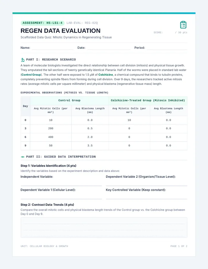
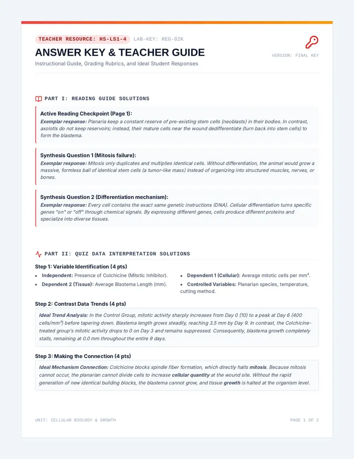
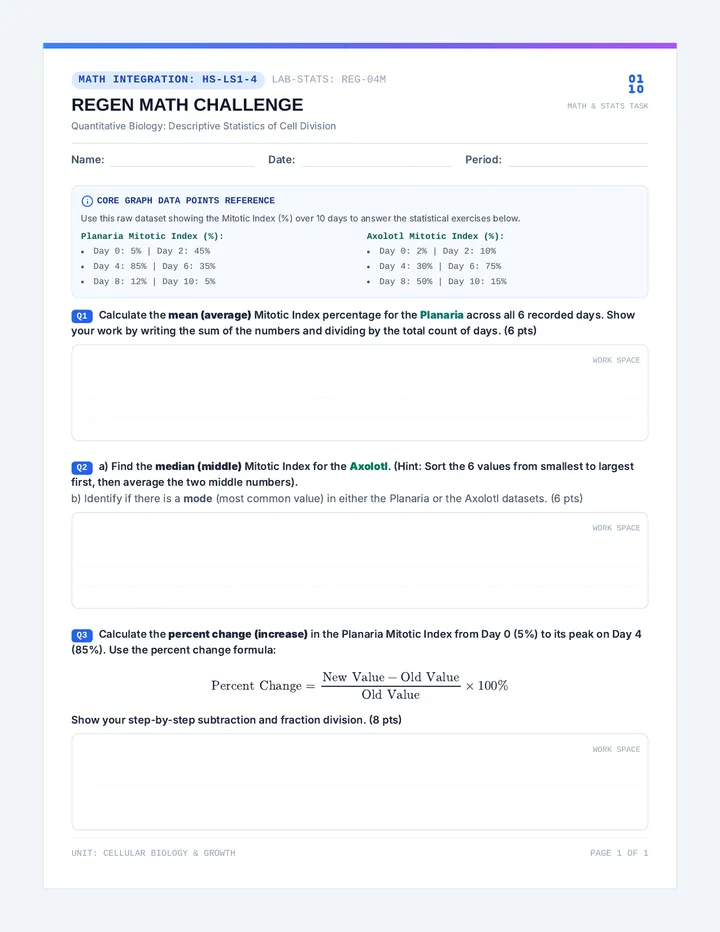
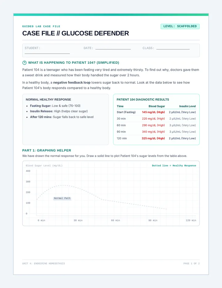
System Dynamics Slides System Dynamics Setup
L1: Equations of Motion for Coupled Masses
The Challenge
How do we describe the motion when the force on one mass depends on the position of another?
"The behavior of the whole is more than the sum of its parts."
m1
m2
2 Masses, 3 Springs: A classical coupled system.
Newton's 2nd Law in Coupling
For Mass 1:
Forces from left spring and middle spring:
\[ m_1 \ddot{x}_1 = -k_1 x_1 + k_2(x_2 - x_1) \]
For Mass 2:
Forces from middle spring and right spring:
\[ m_2 \ddot{x}_2 = -k_2(x_2 - x_1) - k_3 x_2 \]
Crucial Sign Convention
The term \( (x_2 - x_1) \) represents the relative displacement .
If \( x_2 > x_1 \), the middle spring is stretched.
A stretched middle spring pulls \( m_1 \) to the right (+ force).
A stretched middle spring pulls \( m_2 \) to the left (- force).
The Matrix Leap
To solve for many masses, we consolidate these separate equations into a single matrix equation:
\[ \mathbf{M} \mathbf{\ddot{x}} = -\mathbf{K} \mathbf{x} \]
Mass Matrix \( \mathbf{M} \)
\[ \begin{pmatrix} m_1 & 0 \\ 0 & m_2 \end{pmatrix} \]
Diagonal for discrete masses.
Stiffness Matrix \( \mathbf{K} \)
\[ \begin{pmatrix} k_1 + k_2 & -k_2 \\ -k_2 & k_2 + k_3 \end{pmatrix} \]
Off-diagonal terms represent the coupling.
Molecular Vibrations
This isn't just for blocks on strings. This is how we model molecules like Carbon Dioxide (CO₂) .
Atoms = Masses
Chemical Bonds = Springs
Coupling = Shared forces between bonded atoms
O
C
O
System Setup Workshop System Setup Workshop
Lesson 1: Equations of Motion for Coupled Masses
Name:
Date:
Goal: Derive and matrix-formulate the equations of motion for various mass-spring configurations.
1 The Standard System
Consider two masses \( m_1 \) and \( m_2 \) on a frictionless surface. \( m_1 \) is connected to a wall by spring \( k_1 \). \( m_1 \) and \( m_2 \) are connected by spring \( k_2 \). \( m_2 \) is connected to a wall by spring \( k_3 \).
A) Draw the Free Body Diagram (FBD) for both masses when they are displaced such that \( x_2 > x_1 > 0 \). Label all forces with their spring constants and displacements.
FBD for m1
FBD for m2
B) Write the Newton's 2nd Law equations for each mass:
\( m_1 \ddot{x}_1 = \)
\( m_2 \ddot{x}_2 = \)
2 The Matrix Transformation
Rewrite your equations from Section 1 in the form \( \mathbf{M} \mathbf{\ddot{x}} = -\mathbf{K} \mathbf{x} \), where \( \mathbf{x} = \begin{pmatrix} x_1 \\ x_2 \end{pmatrix} \).
M
\[ \begin{pmatrix} \ddot{x}_1 \\ \ddot{x}_2 \end{pmatrix} \]
= —
K
\[ \begin{pmatrix} x_1 \\ x_2 \end{pmatrix} \]
Challenge Question:
What happens to the matrix \( \mathbf{K} \) if the central coupling spring is removed (\( k_2 = 0 \))? What does this mean physically for the system?
3 Scaling Up
Imagine 3 identical masses (\( m \)) and 4 identical springs (\( k \)) in a line between two walls. Sketch the system and predict the size of the \( \mathbf{K} \) matrix.
Sketch area
Size of K matrix:
Number of coupling terms (off-diagonals):
Coupling Equations Guide Coupling Equations Guide
Teacher Resource • Lesson 1: Equations of Motion
Instructional Intent
This lesson bridges the gap between single-oscillator dynamics and multi-variable systems. The goal is to move students away from thinking of "two problems" and toward "one system" described by a vector space.
Key Pedagogical Pivot
Students often struggle with the sign of the coupling force. Emphasize that \( k_2(x_2 - x_1) \) is the extension. If \( x_2 > x_1 \), the spring pulls \( m_1 \) forward (+) and \( m_2 \) backward (-). This Newton's 3rd Law symmetry is reflected in the symmetric off-diagonal terms of the \( \mathbf{K} \) matrix.
Pacing (50m)
Hook & Demo 10m
Derivation (Slides) 15m
Workshop Activity 20m
Closing Discussion 5m
Matrix Solution Key
Newton's 2nd Law (Standard Case)
\[ m_1 \ddot{x}_1 = -k_1 x_1 + k_2(x_2 - x_1) \] \[ m_2 \ddot{x}_2 = -k_2(x_2 - x_1) - k_3 x_2 \]
Common Error: Using \( (x_1 - x_2) \) for both, violating Newton's 3rd Law.
The Stiffness Matrix \( \mathbf{K} \)
\[ \mathbf{K} = \begin{pmatrix} k_1 + k_2 & -k_2 \\ -k_2 & k_2 + k_3 \end{pmatrix} \]
Diagonal: Sum of all springs connected to that mass.
Off-Diagonal: Negative of the coupling spring constant.
Prompt: Physical Intuition
"If \( m_1 \) is fixed in place (\( x_1 = 0 \)), what effective spring constant does \( m_2 \) feel? How does this relate to the entry \( K_{22} \)? Why?"
Differentiation Tip
For advanced students, ask them to write the matrices for a circular chain of 3 masses where the 1st and 3rd are also coupled. This introduces non-zero terms in the top-right and bottom-left corners.
Eigenvalue Essence Slides Eigenvalue Essence
Lesson 2: Finding Normal Modes & Eigenfrequencies
Decoding the "DNA" of mechanical systems.
The Trial Solution (Ansatz)
We assume that every mass in the system oscillates at the same frequency \( \omega \) but with different amplitudes.
\[ \mathbf{x}(t) = \mathbf{a} e^{i \omega t} \]
Where \( \mathbf{a} \) is a vector of amplitudes (the mode shape) and \( \omega \) is the characteristic frequency.
The Substitution
Substituting into \( \mathbf{M} \mathbf{\ddot{x}} = -\mathbf{K} \mathbf{x} \):
\[ -\omega^2 \mathbf{M} \mathbf{a} = -\mathbf{K} \mathbf{a} \]
Rearranging into the standard Eigenvalue problem:
\[ (\mathbf{K} - \omega^2 \mathbf{M}) \mathbf{a} = 0 \]
The Characteristic Equation
For a non-trivial solution (\( \mathbf{a} \neq 0 \)), the matrix must be singular:
\[ \det(\mathbf{K} - \omega^2 \mathbf{M}) = 0 \]
Step 1
Calculate the determinant as a polynomial in \( \omega^2 \).
Step 2
Solve for the roots \( \omega_1^2, \omega_2^2, \dots \)
Physical Interpretation
Each root \( \omega_n \) is an Eigenfrequency . It is a natural frequency at which the system "prefers" to vibrate.
Note
A system with \( N \) degrees of freedom has exactly \( N \) normal modes.
Normal Modes: The In and The Out
In-Phase (Symmetric)
Mode 1
The masses move together. The central coupling spring is neither stretched nor compressed. Frequency is typically lower.
Out-of-Phase (Anti-Symmetric)
Mode 2
The masses move in opposite directions. The coupling spring is heavily involved. Frequency is higher due to extra restoring force.
Matrix Mastery Worksheet Matrix Mastery
Lesson 2: Frequencies and Eigenvectors
Theoretical Physics Lab
Name:
System Parameters
Consider a symmetric system: two identical masses \( m \) connected to outer walls by springs with constant \( k \), and connected to each other by a coupling spring with constant \( \kappa \).
\[ \mathbf{M} = \begin{pmatrix} m & 0 \\ 0 & m \end{pmatrix}, \quad \mathbf{K} = \begin{pmatrix} k+\kappa & -\kappa \\ -\kappa & k+\kappa \end{pmatrix} \]
1. Eigenfrequencies
Set up the characteristic equation \( \det(\mathbf{K} - \omega^2 \mathbf{M}) = 0 \) and show your work to find the two roots for \( \omega^2 \).
\( \omega_1^2 = \)
\( \omega_2^2 = \)
2. Normal Modes (Eigenvectors)
For each frequency found above, solve the equation \( (\mathbf{K} - \omega_n^2 \mathbf{M}) \mathbf{a}_n = 0 \) to find the corresponding eigenvector \( \mathbf{a}_n \). Normalize such that the first entry is 1.
For \( \omega_1^2 \):
\( \mathbf{a}_1 = \)
\[ \begin{pmatrix} 1 \\ \dots \end{pmatrix} \]
For \( \omega_2^2 \):
\( \mathbf{a}_2 = \)
\[ \begin{pmatrix} 1 \\ \dots \end{pmatrix} \]
3. Physical Interpretation
Describe the physical motion associated with each mode. Which frequency is higher and why does that make physical sense in terms of spring restoring forces?
Mode Shape Key Resource Mode Shape Key
Teacher Reference • Lesson 2: Normal Modes
Solutions Guide
Core Insight
The eigenvalues represent the squares of the frequencies (\( \omega^2 \)). The eigenvectors represent the spatial configuration of the system during oscillation. In a normal mode, every part of the system passes through the equilibrium position at the same time.
Common Pitfalls
Students forgetting to square root the eigenvalues to find \( \omega \).
Confusion when normalization produces \( \pm 1 \).
Missing the fact that \( \kappa \) cancels out in the first mode.
1. Eigenfrequency Solutions
\[ \det \begin{pmatrix} (k+\kappa) - m\omega^2 & -\kappa \\ -\kappa & (k+\kappa) - m\omega^2 \end{pmatrix} = 0 \]
Mode 1 (Symmetric)
\[ \omega_1^2 = \frac{k}{m} \]
The coupling spring is not stretched. The system behaves like two independent oscillators.
Mode 2 (Anti-Symmetric)
\[ \omega_2^2 = \frac{k + 2\kappa}{m} \]
The coupling spring is compressed/stretched double the displacement, adding significant restoring force.
2. Eigenvector Interpretation
a₁:
\[ \begin{pmatrix} 1 \\ 1 \end{pmatrix} \]
In-phase: Masses move together.
a₂:
\[ \begin{pmatrix} 1 \\ -1 \end{pmatrix} \]
Anti-phase: Masses move opposite.
Discussion Hook
"Why does Mode 2 have a higher frequency? Connect this to the 'stiffness' the system feels in each configuration."
Mode Mashup Slides Mode Mashup
Lesson 3: Linear Superposition & General Solutions
Building complex reality from simple building blocks.
The General Solution
Since the equations of motion are linear , any linear combination of normal modes is also a valid solution.
\[ \mathbf{x}(t) = \sum_{n=1}^N \mathbf{a}_n \left( A_n \cos(\omega_n t) + B_n \sin(\omega_n t) \right) \]
Degrees of Freedom
A 2-mass system has 4 unknowns to solve for:
\( A_1, B_1 \) (for Mode 1)
\( A_2, B_2 \) (for Mode 2)
These coefficients are determined entirely by the starting state of the system.
Determining the Coefficients
At \( t = 0 \) (Position)
\[ \mathbf{x}(0) = \sum A_n \mathbf{a}_n \]
At \( t = 0 \) (Velocity)
\[ \mathbf{\dot{x}}(0) = \sum \omega_n B_n \mathbf{a}_n \]
The Projection Strategy
Because normal modes are orthogonal (with respect to the mass matrix), we can "pick out" coefficients one by one.
\[ A_n \propto \mathbf{a}_n^T \mathbf{M} \mathbf{x}(0) \]
Example: Pulling one mass
Initial State
Mass 1 is pulled by \( L \), Mass 2 is held at equilibrium.
\[ \mathbf{x}(0) = \begin{pmatrix} L \\ 0 \end{pmatrix} \]
What happens next?
50%
Mode 1 Amplitude
\( A_1 = L/2 \)
50%
Mode 2 Amplitude
\( A_2 = L/2 \)
Both modes are excited equally! The resulting motion will look like "beating" or energy transfer.
General Solution Workshop General Solution Workshop
Lesson 3: Superposition & Coefficients
NAME:
Quantum & Waves Lab
Recall: Normal Modes of Symmetric System
Mode 1
\( \omega_1 = \sqrt{k/m} \)
\( \mathbf{a}_1 = \begin{pmatrix} 1 \\ 1 \end{pmatrix} \)
Mode 2
\( \omega_2 = \sqrt{(k+2\kappa)/m} \)
\( \mathbf{a}_2 = \begin{pmatrix} 1 \\ -1 \end{pmatrix} \)
The General Form
\( \mathbf{x}(t) = A_1 \mathbf{a}_1 \cos(\omega_1 t) + A_2 \mathbf{a}_2 \cos(\omega_2 t) \)
Assuming zero initial velocity for simplicity.
1 Single-Mass Pull
Suppose at \( t=0 \), you displace Mass 1 by a distance \( L \) to the right and hold Mass 2 at its equilibrium position. You release the system from rest.
Write the initial position vector \( \mathbf{x}(0) \):
\[ \begin{pmatrix} \dots \\ \dots \end{pmatrix} \]
Write the initial velocity vector \( \mathbf{\dot{x}}(0) \):
\[ \begin{pmatrix} \dots \\ \dots \end{pmatrix} \]
Show your work solving for \( A_1 \) and \( A_2 \):
2 Selective Excitation
How would you need to displace the masses at \( t=0 \) to ensure that the system oscillates only in Mode 2 (the anti-symmetric mode)?
If you achieve this state, what will the displacement of Mass 1 be at time \( t = \pi / \omega_2 \)? (Provide in terms of the initial displacement \( L \)).
3 The Motion Trace
Given \( \mathbf{x}(t) = \frac{L}{2} \begin{pmatrix} 1 \\ 1 \end{pmatrix} \cos(\omega_1 t) + \frac{L}{2} \begin{pmatrix} 1 \\ -1 \end{pmatrix} \cos(\omega_2 t) \), write an expression for \( x_1(t) \) and \( x_2(t) \) separately using the cosine addition formula \( \cos(A)\cos(B) \) or similar identities if helpful.
\( x_1(t) = \)
\( x_2(t) = \)
Initial Conditions Cheat Sheet Initial Conditions Guide
Teacher Reference • Lesson 3: Superposition
Coefficients & Projections
Guiding the Mathematics
The shift from individual mode solutions to the general solution is conceptually difficult. Help students see that A₁ and A₂ are just the "coordinates" of the initial displacement in the "basis" of the normal modes.
"Just like a vector can be broken into x and y components, any complex motion can be broken into Normal Mode components."
Initial Velocity Alert
Most textbooks focus on position-only starts. Remind students that if they kick the masses (giving them velocity), they must solve for the sine terms:
\[ B_n = \frac{\dot{x}(0) \cdot \mathbf{a}_n}{\omega_n (\mathbf{a}_n \cdot \mathbf{a}_n)} \]
Note: The denominator involves the frequency—higher modes need more 'punch' for the same coefficient.
Workshop Key (Problem 1)
Initial Displacement \( \mathbf{x}(0) = \begin{pmatrix} L \\ 0 \end{pmatrix} \)
Using the symmetry of the eigenvectors \( \mathbf{a}_1 = (1, 1)^T \) and \( \mathbf{a}_2 = (1, -1)^T \):
\[ \begin{pmatrix} L \\ 0 \end{pmatrix} = A_1 \begin{pmatrix} 1 \\ 1 \end{pmatrix} + A_2 \begin{pmatrix} 1 \\ -1 \end{pmatrix} \]
\[ A_1 = L/2, \quad A_2 = L/2 \]
Selective Excitation (Problem 2)
To get Mode 2 only, set \( \mathbf{x}(0) \propto \mathbf{a}_2 \).
Action: Displace masses by equal amounts in opposite directions (\( x_1 = L, x_2 = -L \)).
The Trig Identity (Problem 3)
\[ x_1(t) = L \cos\left(\frac{\omega_1+\omega_2}{2}t\right) \cos\left(\frac{\omega_2-\omega_1}{2}t\right) \]
This is the math behind the "beats" they will study in Lesson 4!
Pulse Patterns Slides Pulse Patterns
Lesson 4: Beating and Weak Coupling
The slow dance of energy exchange.
When Coupling is Weak
In a weakly coupled system, the interaction spring is much softer than the main springs:
\[ \kappa \ll k \]
This results in two normal mode frequencies that are very close to each other: \( \omega_1 \approx \omega_2 \).
The Consequence
When two nearly identical frequencies interfere, we don't hear (or see) two separate tones. We see a single oscillation whose amplitude is modulated .
The Beat frequency
Adding the modes for Mass 1:
\[ x_1(t) = A \cos\left(\frac{\omega_1+\omega_2}{2}t\right) \cos\left(\frac{\omega_2-\omega_1}{2}t\right) \]
Average Frequency: Rapid oscillation.
Modulation Frequency: Slow variation.
The Envelope
The amplitude is defined by the slow term. The energy in the mass "beats" with a period defined by:
\[ \omega_{beat} = |\omega_2 - \omega_1| \]
The Paradox of Energy Transfer
When Mass 1 is stationary at equilibrium, Mass 2 has maximum amplitude.
The coupling spring "pumps" energy from one oscillator to the other. Because they are the same mass, they can exchange 100% of their energy.
"It’s like a mechanical conversation where only one person can speak at a time."
Max Amplitude
Stationary
Energy at t = 0
Beat frequency Investigation Beat frequency Investigation
Lesson 4: Envelope Analysis & Trig Derivation
Physics Core Lab
STUDENT ID:
"When we listen to a guitar being tuned, we hear 'beats'—a pulsing volume. Today we derive the mathematics of that pulse from first principles of coupled motion."
1 The Superposition Identity
Given the position of Mass 1 for a symmetric start: \( x_1(t) = A\cos(\omega_1 t) + A\cos(\omega_2 t) \).
Use the sum-to-product identity: \( \cos(X) + \cos(Y) = 2\cos\left(\frac{X+Y}{2}\right)\cos\left(\frac{X-Y}{2}\right) \) to rewrite \( x_1(t) \).
\( x_1(t) = \)
2 The Slow and the Fast
The "Fast" Frequency:
\[ \omega_{avg} = \]
This determines the pitch or the rapid oscillation.
The "Slow" (Envelope) Frequency:
\[ \omega_{env} = \]
This determines the rate of amplitude modulation.
Question:
If \( \omega_2 = 1.05 \, \text{rad/s} \) and \( \omega_1 = 1.00 \, \text{rad/s} \), how many seconds elapse between points of maximum displacement for Mass 1?
3 Visualizing the Transfer
Sketch the displacement of Mass 1 over a full beat cycle. Include the "envelope" (dotted lines) and the "carrier wave" (solid line).
Time (t)
Displacement (x)
Synthesis Prompt
Explain where the energy from Mass 1 goes when its amplitude reaches zero. If you were looking at the graph for Mass 2, how would it differ from the one you just sketched?
Energy Transfer Guide Energy Transfer Guide
Teacher Reference • Lesson 4: Beating
Weak Coupling Mastery
Instructional Strategy
Students often find "beating" to be a purely mathematical trick. Your goal is to ground it in Conservation of Energy . In a symmetric system, total energy is constant, but it "shuttles" between the two oscillators via the coupling spring.
The "Ah-ha" Moment
Point out that at the center of a beat cycle for Mass 1 (amplitude = 0), Mass 2 is at maximum amplitude . The energy is not lost; it is just "hiding" in the other mass.
Demonstration Tip
Suspend two identical pendulums from a single slightly slack horizontal string.
1. Pull P1 back.
2. Observe P1 stop.
3. Observe P2 peak.
Wilberforce Pendulum Variant
Math Solution Key
Trig Derivation (Problem 1)
Final form after sum-to-product:
\[ x_1(t) = 2A \cos\left(\frac{\omega_1+\omega_2}{2}t\right) \cos\left(\frac{\omega_2-\omega_1}{2}t\right) \]
Beat Period (Problem 2)
Calculation for \( \Delta \omega = 0.05 \):
\( \text{Period} = 2\pi / \Delta \omega = 125.7 \, \text{s} \)
Note: The "beat" heard by the ear is twice this frequency because energy is heard as intensity \( \propto A^2 \).
Deep Inquiry Prompt
"What happens if the masses are slightly different? Will energy still transfer 100%? Why or why not?"
Answer: No. Complete transfer requires resonance. Imbalance limits the 'pumping' efficiency.
Continuum Transition Slides The Continuum Leap
Lesson 5: From Coupled Masses to Waves
Where discrete particles become a single fluid motion.
Generalizing to N Masses
Instead of 2 masses, imagine an infinite chain of identical masses \( m \) separated by spacing \( a \), connected by springs \( k \).
\[ m \ddot{x}_j = k(x_{j+1} - x_j) - k(x_j - x_{j-1}) \]
This is the fundamental equation for the \( j^{th} \) mass.
j
Shrinking the Spacing
As the spacing \( a \to 0 \), the discrete positions \( x_j \) become a continuous variable \( x \).
Finite Difference to Derivative
\[ \frac{(x_{j+1} - x_j) - (x_j - x_{j-1})}{a^2} \approx \frac{\partial^2 \psi}{\partial x^2} \]
The Continuum Limit
Multiplying by mass density \( \rho = m/a \) and tension/stiffness \( Y = ka \), we arrive at the holy grail of mechanics:
\[ \frac{\partial^2 \psi}{\partial t^2} = v^2 \frac{\partial^2 \psi}{\partial x^2} \]
Sound, Strings, and Solids
Guitar Strings
Transverse waves modeled as infinite coupled oscillators under tension.
Crystals
Atoms in a lattice vibrate as coupled systems. Phonons are the Normal Modes of the crystal!
Sound Waves
Air molecules act as masses connected by the "springiness" of pressure.
Discrete physics isn't a simplification—it's the foundation of the continuous world.
Infinity Chain Challenge Infinity Chain Challenge
Lesson 5: Deriving the Wave Equation
Theoretical Mechanics Lab
Collaborators:
In this final workshop, we unify everything we've learned. We will take a chain of \( N \) identical masses and see how, as the system becomes infinite and dense, it transforms into a single continuous medium governed by a partial differential equation.
Part 1: The Discrete Force Law
Consider the \( j^{th} \) mass in a chain. Write the equation of motion for \( \ddot{x}_j \) using only \( x_{j-1}, x_j, x_{j+1} \) and the constants \( m \) and \( k \).
\[ m \ddot{x}_j = \]
Assume a wave solution: \( x_j(t) = A e^{i(k_w ja - \omega t)} \), where \( k_w \) is the wavenumber and \( a \) is the spacing. Substitute this into your equation and solve for \( \omega^2 \).
Math Area
Part 2: Taking the Limit
Let \( a \to 0 \). Using the Taylor expansion \( f(x \pm a) \approx f(x) \pm a f'(x) + \frac{a^2}{2} f''(x) \), show that the discrete force equation from Part 1 becomes:
\[ \frac{\partial^2 \psi}{\partial t^2} = \left( \frac{ka^2}{m} \right) \frac{\partial^2 \psi}{\partial x^2} \]
Identifying Constants:
Define linear mass density \( \mu = m/a \) and Young's Modulus equivalent \( Y = ka \). Rewrite the wave speed \( v \) in terms of \( Y \) and \( \mu \).
\[ v = \]
Final Synthesis
How does the concept of "Normal Modes" apply to a continuous string compared to a 2-mass system? Are there still a finite number of modes? Explain.
Wave Derivation Notes Wave Derivation Notes
Teacher Reference • Lesson 5: Continuum Limit
Formal Derivation Key
The Conceptual Bridge
This is the most mathematically demanding lesson of the sequence. The goal is to show students that differential equations are just the limit of coupled systems . Help them see the second spatial derivative as the "difference of differences" in spring forces.
Taylor Series Reminder
Students often miss why the first-order terms cancel. Emphasize that:
\[ x_{j+1} - x_j \approx a \psi' + \frac{a^2}{2} \psi'' \] \[ x_{j-1} - x_j \approx -a \psi' + \frac{a^2}{2} \psi'' \] Summing these cancels the \( a \psi' \) terms, leaving the second derivative.
Key Derivation Landmarks
1. The Discrete System
\[ m \ddot{\psi}_j = k(\psi_{j+1} - \psi_j) - k(\psi_j - \psi_{j-1}) = k(\psi_{j+1} + \psi_{j-1} - 2\psi_j) \]
2. The Continuum Variables
Remind students to multiply and divide by \( a^2 \) to get the derivative definition:
\[ m \frac{\partial^2 \psi}{\partial t^2} = (ka^2) \left[ \frac{\psi_{j+1} + \psi_{j-1} - 2\psi_j}{a^2} \right] \]
3. The Final Form
Divide by \( a \) to get density on the left:
\[ \frac{m}{a} \frac{\partial^2 \psi}{\partial t^2} = (ka) \frac{\partial^2 \psi}{\partial x^2} \implies \mu \ddot{\psi} = Y \psi'' \]
Closure Discussion Hook
"On a continuous string, every point is a mass. Does this mean there are an infinite number of Normal Modes? If so, what do they look like?"
Answer: Yes! The normal modes are the harmonics (sine waves) that fit the boundary conditions. They represent the transition from matrix eigenvectors to functional eigenfunctions.