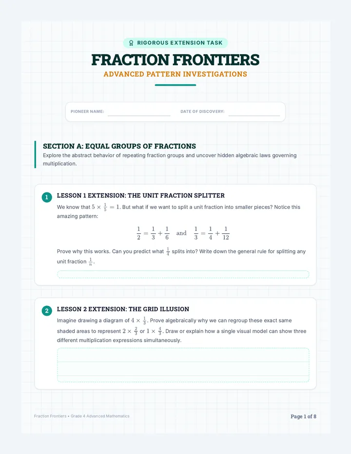
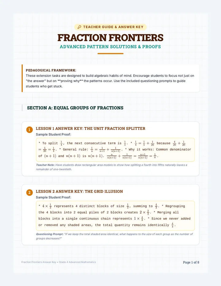
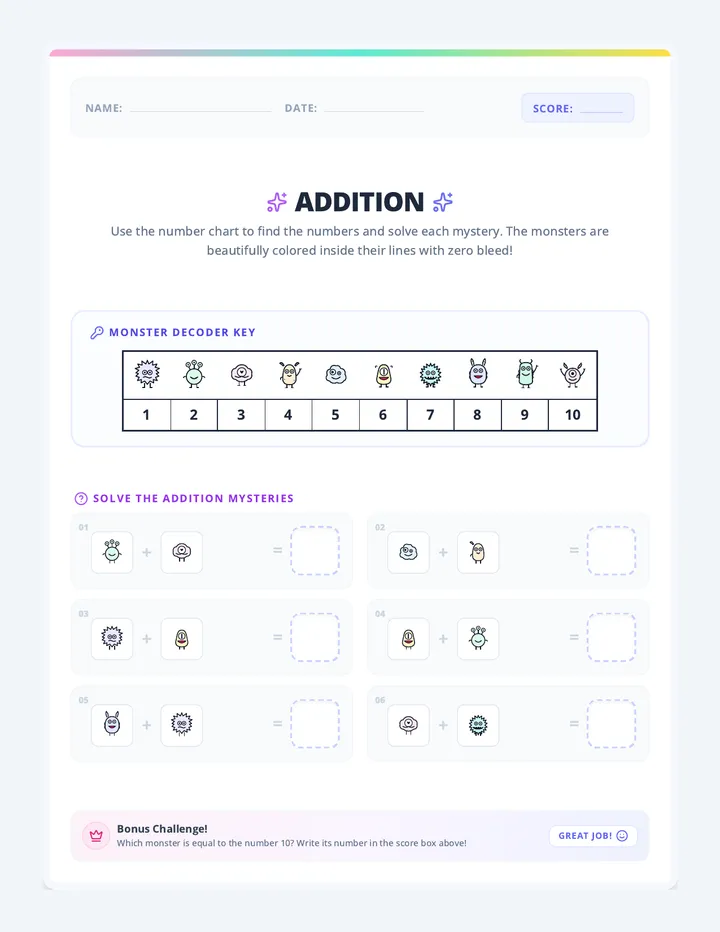
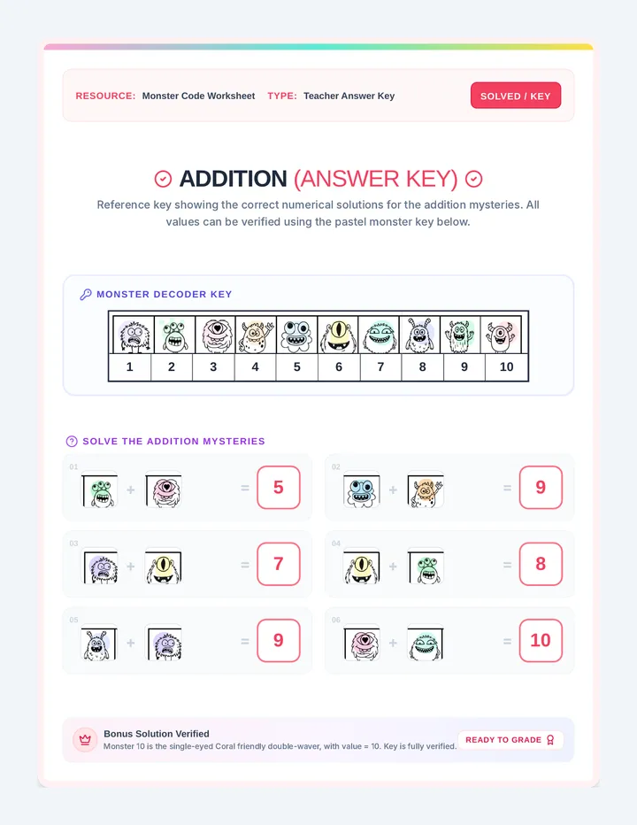
Queueing Essentials Slides Module 01: Stochastic Basics
Queueing Essentials
Decoding the hidden math behind why we wait and how to make lines disappear.
Arrivals (λ)
Service (μ)
Capacity (c)
The Efficiency Paradox
Scenario A: The Grocery Store
Individual lines for each cashier.
You pick a line and stay in it.
One slow customer blocks everyone.
Scenario B: The Bank / Fast Food
One "Snake" line for all servers.
Next person goes to next open window.
A slow customer is bypassed.
"Which system is mathematically superior for wait times?"
The Language of Queues
λ (Lambda)
Arrival Rate
Mean number of customers entering the system per unit of time (e.g., 10 per hour).
μ (Mu)
Service Rate
Mean number of customers a single server can process per unit of time (if busy).
c
Server Count
The number of parallel channels available to process customers.
System Utilization (ρ) = λ / (c * μ)
If ρ ≥ 1, the queue grows infinitely! Stability is key.
Kendall's Notation: A/B/c
A: Arrival Distribution
Usually M (Markovian/Poisson) - meaning arrivals are random and independent.
B: Service Distribution
Usually M (Exponential) - meaning task lengths vary randomly.
c: Number of Servers
1 = Single counter; 5 = Five parallel counters.
Example: M/M/1
One ticket booth. People arrive randomly. Processing time is random. One person served at a time.
1
Example: M/M/3
One waiting line, three open tellers. High efficiency, reduced wait variance.
A
B
C
Case Study: Drive-Thru vs. Dine-In
A fast-food restaurant has two servers. One handles the drive-thru exclusively, the other handles walk-in customers.
The Challenge:
"If the drive-thru is empty but the lobby is packed, one server sits idle. How does merging the queues change the system's λ and μ?"
Queueing Analysis Worksheet Queueing System Analysis
Worksheet // Stochastic Modeling
Student Name:
Class Period:
1
Anatomy of a Queue
Analyze the following scenario and identify the key parameters using standard stochastic notation. Scenario: A local health clinic has 3 nurses who perform flu vaccinations. Patients arrive at an average rate of 12 per hour. On average, a nurse takes 10 minutes to process one patient.
λ (Arrival Rate)
per hour
μ (Service Rate per Server)
per hour
c (Server Count)
// SYSTEM UTILIZATION (ρ)
Formula: λ / (c * μ)
Calculate ρ for this clinic. What does this value tell us about the stability of the queue?
2
Queue Topologies
Design 1: M/M/1 System
Draw a diagram representing a single-server system. Label the Input Source , Queue , Service Mechanism , and Departures .
[Student Workspace]
Design 2: M/M/3 System
Draw a diagram representing a system with 3 parallel servers and 1 shared waiting line. Identify where λ and μ apply.
[Student Workspace]
3
Optimization Challenge
The "Pooling" Effect
Suppose a grocery store has two checkout lanes, each with its own line. Lane A and Lane B both have identical arrival rates (λ = 10/hr) and service rates (μ = 12/hr). The store manager decides to "pool" the lines into a single snake-line that feeds both registers (converting two M/M/1 systems into one M/M/2 system).
Will the total average wait time for a customer decrease, increase, or stay the same? Explain your reasoning using the concept of variance.
System Stress Test
If the arrival rate (λ) suddenly doubles for the flu clinic from Part 1, but the number of nurses remains 3, what is the new ρ? Is the system still stable? If not, what is the minimum number of nurses needed to return to a stable state (ρ < 1)?
Queueing Teacher Guide Teacher Guide
Lesson 1: Introduction to Queueing
Queueing Essentials
Facilitating the transition from static probability to dynamic systems.
Learning Objectives
Define and identify $\lambda$, $\mu$, and $c$ in real-world scenarios.
Use Kendall's Notation ($A/B/c$) to classify service systems.
Calculate system utilization ($\rho$) and assess system stability.
Qualitatively explain the "pooling effect" in queueing topology.
Lesson Pacing
10m
The Hook: Drive-Thru Paradox
Show a video/photo of a crowded store. Ask: "Why is the longest line sometimes the fastest?"
20m
Direct Instruction: The Parameters
Introduce $\lambda, \mu, c$ and $\rho$. Use the slides to visualize $M/M/1$ vs $M/M/c$.
20m
Guided Practice: Queueing Worksheet
Students work through the analysis of the health clinic and topology sketching.
10m
Debrief: The Pooling Effect
Group discussion on why the "snake line" is mathematically superior despite appearing longer.
Key Discussion Prompts
"If arrivals are random, what happens to the line when three people arrive at once by pure chance?"
"Why is system utilization over 100% physically impossible in the long run?"
"Think of a system where 'pooling' doesn't work. Why? (e.g., highly specialized medical specialists)."
Answer Key: Queueing Analysis
Part 1: The Health Clinic
λ: 12 patients/hour.
μ: 6 patients/hour (since 10 mins/patient = 60/10).
c: 3 nurses.
ρ: $12 / (3 * 6) = 12 / 18 = 0.67$ (or 67%).
Stability: Stable. The system is utilized at 67%, meaning nurses are idle about 33% of the time, providing a buffer for random bursts.
Part 3: The Pooling Effect
Wait time will decrease. In individual lines, if one server gets a "difficult" customer (high variance in service time), that line stalls while others remain empty. In a pooled $M/M/2$ system, the difficult customer only occupies one server, while the other server continues to process the shared queue. This reduces the probability of a server being idle while customers are waiting.
Part 3: Stress Test
New λ: 24 patients/hour.
$24 / (3 * 6) = 24 / 18 = 1.33$ (133%).
Monte Carlo Logic Slides Module 02: Monte Carlo Methods
Monte Carlo Logic
Harnessing randomness to solve the unsolvable through millions of virtual experiments.
Random Sampling
Large Scale Trials
Statistical Inference
How to calculate π with a dartboard?
1. Draw a circle inside a square.
2. Throw 10,000 darts randomly at the square.
3. Count how many land inside the circle.
π ≈ 4 × (Darts In Circle / Total Darts)
R
Picking Your Randomness
Uniform
Every outcome is equally likely. Good for choosing a "random spot" on a map.
Normal (Gaussian)
Bell curve. Good for human traits, heights, or small errors in measurements.
Exponential
High probability of low values. Crucial for time between arrivals in queues.
The Simulation Engine Loop
Step 1: Input
Generate a random value from your chosen distribution.
Step 2: Process
Apply the logic (e.g., If Arrival Time < Service End Time, person waits).
Step 3: Accumulate
Store the result and repeat for N = 10,000 trials.
"We aren't looking for a single answer. We are looking for the distribution of possible answers."
Simulation Blueprint Worksheet Simulation Blueprint
Design Phase // Project: Stochastic Modeling
Phase 01: Architecture
Name: __________________________ Date: __________________________
01
Scenario Definition
Choose a real-world system to model (e.g., a coffee shop, a security checkpoint, a server farm, or a traffic light). Describe the problem you want to solve.
Primary Objective
What metric are you trying to optimize? (e.g., minimize wait time, maximize server usage)
Constraints
What limits the system? (e.g., budget for employees, physical space for queueing)
02
Random Variables & Distributions
Variable Name Distribution Type Rationale / Estimated Parameters
*Distributions include: Uniform, Normal, Exponential, Poisson, etc.
03
Simulation Logic (Pseudocode)
Draft the step-by-step logic for one single trial of your simulation. How does the system state change from "Arrival" to "Departure"?
// Example Template:
1. Generate random inter-arrival time (t_arr)
2. Clock_Time = Clock_Time + t_arr
3. Determine if server is available...
4. [Your Logic Here]
// Write your logic below:
Building the Engine Slides Module 03: Implementation
Building the Engine
Translating logic into code. Creating the clock, the arrivals, and the state-trackers.
The Three Pillars of a Simulator
The Clock
Manages time progression. Does your simulation jump by fixed time steps (0.1s) or by the next discrete event (Arrival/Departure)?
The RNG
Random Number Generator. Converts 0-1 uniform noise into the distributions (Exponential, Normal) you identified in your blueprint.
The State
Tracks variables like queue_length, server_busy, and total_wait_time.
Essential Spreadsheet Functions
Your toolset for Monte Carlo in Excel or Sheets.
=RAND()
Generates a uniform random number between 0 and 1.
=NORM.INV(RAND(), mean, std_dev)
Converts a random seed into a Normal Distribution value.
=-LN(RAND()) / λ
Inverse Transform Sampling for an Exponential Distribution (Wait times).
=IF(server_free, "Serve", "Wait")
Conditional logic for state changes.
Phase 3: The Build
1
Setup your columns: Arrival Time, Service Duration, Start Time, Wait Time, End Time.
2
Implement the math for Row 2 (the first customer).
3
Define the logic for Row 3: It must reference Row 2 (the "Previous state").
4
"Drag Down" to simulate 1,000 customers. Observe the random patterns.
Coder Challenge
"If you are using Python, initialize a list for your outcomes and use a for loop to run your simulation function N times."
Simulation Dev Kit Reference Simulation Dev-Kit
Syntax & Logic Cheat Sheet
Generating Randomness
Excel / Google Sheets
Uniform (0,1)
=RAND()
Normal (μ, σ)
=NORM.INV(RAND(), mean, std_dev)
Exponential (λ)
=-LN(RAND()) / lambda
Python (random library)
Uniform (0,1)
random.random()
Normal (μ, σ)
random.gauss(mu, sigma)
Exponential (λ)
random.expovariate(lambda)
System State Logic
For a sequential simulation (where rows represent customers), use these logical connections to determine how one customer's timing affects the next.
Arrival Time
Logic: [Previous Customer's Arrival] + [Inter-Arrival Random Jump]
Service Start
Logic: MAX(Arrival Time, Previous Customer's Departure Time).
A customer cannot start until they arrive AND the server is free.
Wait Time
Logic: [Service Start] - [Arrival Time]
Departure Time
Logic: [Service Start] + [Random Service Duration]
Debugging Checklist
Are your time units consistent? (Don't mix minutes and seconds).
Is your wait time ever negative? (If so, check your MAX function).
Are you using λ (rate) instead of 1/λ (average time) in your RNG?
Does the queue grow to thousands of customers immediately? (Check if ρ > 1).
Data Harvest Slides Module 04: Data Analysis
Data Harvest
Running the trials, aggregating the results, and finding the signal in the stochastic noise.
The Law of Large Numbers
A single simulation run is just one "possibility." To find the truth , we must run it N times.
"As the number of trials increases, the experimental mean approaches the theoretical expected value."
n → ∞ μexp ≈ μtheory
Wait Time Distribution (N=10,000)
What are we measuring?
Wq: Average Wait in Queue
How long does the average customer wait before service begins?
Metric: AVERAGE(Wait_Times)
Lq: Average Queue Length
How many people are standing in line on average? Crucial for physical space planning.
Metric: MEAN(People_Waiting_Count)
P95: 95th Percentile Wait
The "worst case" scenario. How long do the unluckiest 5% wait?
Metric: PERCENTILE.INC(Wait_Times, 0.95)
ρactual: Realized Utilization
What percentage of the simulation time were the servers actually busy?
Metric: (Total_Service_Time / Total_Run_Time)
Sensitivity Analysis
Now that your model works, you must find the breaking point . Change your variables and watch the output shift.
Input
Add 1 Server
- 40% Wait
Win!
Input
+10% Arrivals
+ 300% Wait
Crash!
Trial Tracker Worksheet Trial Tracker & Output Analysis
Experimental Phase // Stochastic Modeling
RUN_ID: SIM_X44
SUBJECT: __________________
01
Baseline Statistics (Trial N=1,000+)
Run your simulation for a minimum of 1,000 agents. Calculate the aggregate metrics for your "Current System" (as it exists today).
Avg. Wait Time (Wq)
Max Wait Time
System Utilization (ρ)
Distribution Sketch
Create a rough histogram sketch of your Wait Times . Mark the mean and the 95th percentile.
[Workspace: Draw histogram of wait times here]
02
Sensitivity Analysis
Systematically change one input variable at a time and record the impact on system performance.
Modification Change in λ or μ New Avg. Wait (Wq) % Impact Scenario A: (e.g., +1 Server) Scenario B: (e.g., Rush Hour) Scenario C: (Custom)
03
Critical Observations
The Breaking Point
At what input value does your system stop being stable? How close is the current baseline to this edge?
Unexpected Outcomes
Did any modification have a disproportionately large (or small) effect? Explain using the concept of non-linear behavior in queues.
Optimization Presentation Slides Module 05: Presentation
Optimization Mastery
From raw data to executive decisions. Communicating complex stochastic findings with clarity and impact.
Structure of an Analysis Report
1. The Model
Scenario, assumptions, and Kendall notation ($A/B/c$).
2. The Baseline
Current performance metrics and wait time distributions.
3. The Tests
Sensitivity results: How changes in $\lambda$ and $\mu$ impacted the system.
4. Recommendation
Concrete steps for optimization based on data.
Crafting a Recommendation
Don't just show data. Make a Data-Driven Case .
Weak Recommendation
"Wait times are long, so we should hire more people."
Strong Recommendation
"Adding a 3rd server reduces 95th percentile wait from 15m to 4m, while maintaining a stable ρ of 0.82."
Executive Summary Tips
Highlight the "Crash Point."
Consider Cost vs. Benefit.
Focus on Human Impact.
The Final Showcase
Duration
5 Minutes
Visuals
Charts + Logic Flow
Q&A
2 Minutes Defense
"Your goal is to convince the 'System Manager' that your solution is both efficient and robust."
Optimization Project Rubric Simulation Project Rubric
Assessment Resource // Stochastic Modeling
TOTAL: 100 PTS
Criteria Exemplary (20) Proficient (15) Developing (10) Model Architecture
Identification of λ, μ, and distribution types.
| Distributions (Exponential, etc.) are correctly applied with clear mathematical justification. | Variables are correctly identified, but distribution selection lacks depth or minor errors in parameters. | Variable parameters are incorrect or missing; distribution logic is flawed. |
|
Technical Build
Engine logic, RNG accuracy, and state tracking.
| Simulation engine is robust; handles queue states (Max functions, logical branches) flawlessly. | Simulation works correctly for most trials; minor logical errors in edge cases (e.g., negative waits). | Simulation logic has significant errors; engine does not represent a valid stochastic process. |
|
Statistical Analysis
Percentiles, means, and sensitivity tests.
| Exceptional use of metrics (P95, ρ). Sensitivity analysis clearly identifies system "breaking point." | Basic metrics (mean, max) are calculated correctly. Sensitivity analysis is present but shallow. | Analysis is limited to basic averages; no exploration of variance or outliers. |
|
Recommendations
Actionable insight derived from simulation data.
| Recommendations are highly specific, data-backed, and consider realistic trade-offs. | Recommendation is supported by data but lacks specific impact metrics or cost-benefit reasoning. | Recommendation is generic or not clearly linked to the simulation results. |
|
Communication
Visual clarity and technical defense.
| Visuals (histograms/charts) are professional. Defends model logic with deep technical confidence. | Visuals are clear. Responds well to questions but may struggle with deep technical edge cases. | Visuals are cluttered or missing key labels. Defense is purely descriptive rather than analytical. |
Instructor Feedback
Final Calculation
___ / 100
Validated Score