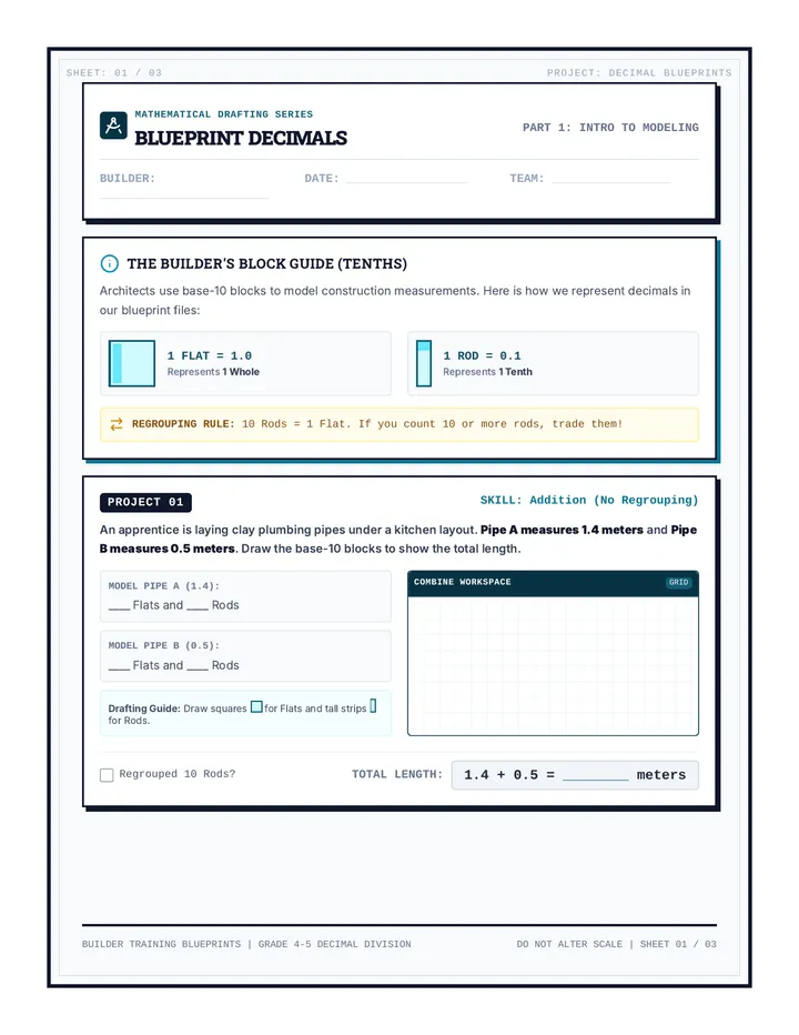
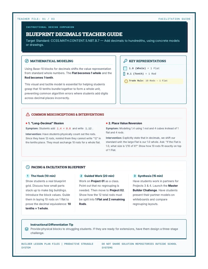
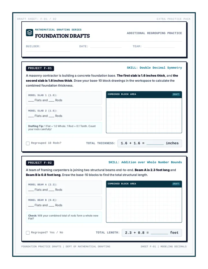
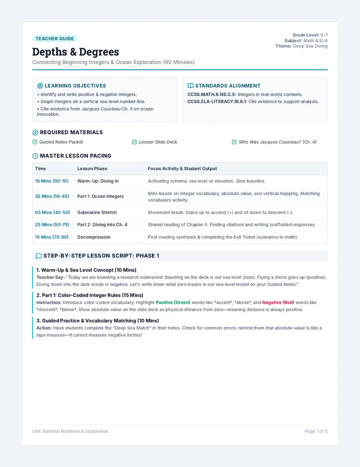
Tradeoff Visuals Slides Lab 01: Foundations
The Bias-Variance Tradeoff
Visualizing the tension between model simplicity and complexity in predictive modeling.
The Ultimate Goal
Generalization
"We don't care how well a model fits the data we have . We care how well it predicts the data we don't have yet."
Training Set: Data used to build the model.
Test Set: Unseen data used to evaluate performance.
The Generalization Gap
The difference between Training Error and Testing Error is our primary diagnostic for model health.
Underfitting: High Bias
Low Complexity
Definition
The model is too simple to capture the underlying structure of the data. It makes strong, but incorrect, assumptions about the data shape.
Symptoms
High Training Error
High Testing Error
A linear model trying to fit a quadratic process.
Overfitting: High Variance
High Complexity
Definition
The model is so flexible that it "memorizes" the noise (random fluctuations) in the training data rather than the actual signal.
Symptoms
Low Training Error
High Testing Error
A 10th-degree polynomial fitting noise in a 2nd-degree process.
The Bias-Variance Tradeoff
Optimal Complexity
Error
Model Complexity
Training Error Total Error (Test)
Sweet Spot
LEFT SIDE
High Bias
Total error is dominated by bias. Both errors are high.
RIGHT SIDE
High Variance
Total error is dominated by variance. Test error diverges.
The Goal
Minimize Total Error by finding the complexity where \( \text{Error} = \text{Bias}^2 + \text{Variance} + \text{Noise} \).
Simulation Facilitation Guide Simulation Guide
Module 01: Bias-Variance Tradeoff
TEACHER RESOURCE
Instructional Goal
Students will use a polynomial regression simulation (using Python/Jupyter, R/Shiny, or an interactive web app) to observe how increasing the degree of a polynomial reduces training error while causing test error to fluctuate and eventually skyrocket.
Simulation Parameters
Data Generation
True Function: \( y = \sin(x) + \epsilon \)
Domain: \( [0, 2\pi] \)
Sample Size: 20 points (Training), 100 points (Test)
Noise (\(\epsilon\)): Gaussian with \( \sigma = 0.3 \)
Student Tasks
Fit polynomials of degree 1, 3, and 15.
Calculate MSE for both sets.
Plot the degree vs. MSE curve.
Identify the "Optimal Degree".
Facilitation Prompts
1
Observation: The Degree 15 Fit
Ask: "Look at the edges of the plot. Why is the 15th-degree polynomial swinging wildly up and down?"
Key Concept: High variance. The model is chasing individual noise points rather than the sine wave trend.
2
Observation: The Error Divergence
Ask: "At what degree does the test error start increasing? Why does the training error keep going down?"
Key Concept: The model has enough degrees of freedom to pass through every training point, but these 'memorized' paths are irrelevant to new data.
Reference Outcomes
Polynomial Degree Diagnosis Training MSE Testing MSE Degree 1 (Linear) Underfit (High Bias) High (~0.8) High (~0.85) Degree 3-5 Optimal Balance Low (~0.1) Lowest (~0.12) Degree 15+ Overfit (High Variance) Near Zero Extreme (>5.0)
Tradeoff Analysis Worksheet Tradeoff Analysis
Lab 01: Polynomial Regression Simulation
NAME:
DATE:
In this lab, you used a simulation to fit polynomials of varying degrees to noisy data. Use your findings to answer the following questions.
1 Visualizing the Fit
Describe the visual behavior of the degree 1 (linear) model compared to the degree 3 model. Which one appears to "capture the signal" better, and why?
When you increased the degree to 15 or higher , what happened to the line between the data points? Explain this behavior using the term variance .
2 The Error Curve
Sketch the general shape of the Training MSE and Testing MSE as a function of polynomial degree based on your simulation results.
MSE (Error)
Polynomial Degree (Complexity)
Training Error
Testing Error
3 Defining the Tradeoff
The Golden Question
If your goal is to minimize Training MSE, which model should you always choose? Explain why this choice might be a mistake if your goal is prediction on new data.
Based on your simulation, what was the "Optimal Degree"? How did you identify it mathematically?
Resampling Rigor Slides Lab 02: Resampling
Resampling Rigor
Mastering Cross-Validation to estimate real-world model performance.
The Validation Trap
Lucky Splits
The Problem
A single Train-Test split is high variance . Your error estimate depends heavily on which specific points ended up in the test set.
"Is my model actually good, or did I just get an easy test set?"
Data Volatility
Small datasets are particularly prone to "unrepresentative" splits.
Efficiency Loss
In a 70/30 split, 30% of your data is never used to train the model.
k-Fold Cross-Validation
Iterative Testing
Iteration 1
Iteration 2
Iteration 3
Iteration 4
Iteration 5
Step 1: Partition
Split the data into \( k \) equal-sized groups (folds).
Step 2: Iterate
Train on \( k-1 \) folds, test on the remaining fold. Repeat \( k \) times.
Step 3: Average
Combine the results (e.g., mean MSE) for a robust estimate.
Leave-One-Out (LOOCV)
k = n
The Definition
A special case of k-fold where \( k \) equals the number of observations (\( n \)). You train on every point except one, and repeat for every point in the dataset.
Pros
Lowest possible bias
No randomness in results
Cons
Computationally expensive
High variance of estimates
Cost Warning
LOOCV requires training the model n times . For a billion-row dataset, this is impossible.
Choosing k
Standard Practice: k=5 or k=10
The choice of \( k \) is itself a tradeoff:
Low k
Higher Bias / Lower Variance
"The training set is much smaller than the full dataset."
Hi k
Lower Bias / Higher Variance
"Training sets overlap almost entirely."
Key Takeaway
Cross-validation provides a sample of performance estimates. We can use the mean for selection and the standard deviation to measure our confidence in the model's stability.
\( \text{CV}_{(k)} = \frac{1}{k} \sum_{i=1}^{k} \text{MSE}_i \)
CV Implementation Lab Manual CV Implementation Lab
Module 02: Resampling Protocols
STUDENT ID:
Objective
Compare the reliability of error estimates across three validation strategies: a single hold-out split, 5-fold cross-validation, and LOOCV.
The Dataset
You are working with a small dataset (\( n=50 \)) measuring the impact of chemical dosage on crop yield. Because the dataset is small, a single random split might be misleading.
Total Sample
50
Train (70%)
35
Test (30%)
15
Protocol Execution
Simulate the following methods and record your "Test MSE" estimates below.
Method A: Single Random Split
Iteration Count: 1
Calculated MSE
0._____
Risk Check: What happens if the 15 points in your test set are all outliers? How would your MSE change?
Method B: 10-Fold Cross-Validation
Iteration Count: 10
Record the MSE for the first 5 folds:
FOLD 1
FOLD 2
FOLD 3
FOLD 4
FOLD 5
Mean CV Error
0._____
Std. Deviation of Error
0._____
Critical Synthesis
1. Look at the Standard Deviation of your 10-fold CV. What does this number tell you about your model's stability? If it were very high, would you trust your model for production use?
2. Why might LOOCV yield a higher variance in error estimates compared to 10-fold CV, even though it uses more training data per iteration?
Validation Protocol Key Validation Key
Module 02: Resampling Rigor
TEACHER KEY & DISCUSSION GUIDE
Expected Experimental Values
Method A: Single Split
Values will vary wildly by student due to random seed. Use this variability as a teaching moment.
Expected Range: 0.25 to 1.10 MSE
Note: Students with low values will think their model is perfect; those with high values will think it failed.
Method B: 10-Fold CV
Mean CV error should converge toward the "true" out-of-sample error.
Mean MSE: ~0.45
Std Dev: ~0.08
Note: Emphasize that the average is more trustworthy than any single fold's error.
Synthesis Question Key
Q1: What does the Standard Deviation tell you?
Key Answer: It measures stability . A high standard deviation indicates that the model's performance is highly sensitive to the specific training data it receives (High Variance). If the SD is high, we cannot be confident that the model will perform consistently on new data.
Q2: Why does LOOCV have high variance in estimates?
Key Answer: Even though LOOCV has the lowest bias, the training sets in each iteration are almost identical (they share \( n-2 \) points). This makes the outputs of the models highly correlated. The mean of highly correlated variables has a higher variance than the mean of less correlated variables (like those in 5-fold CV).
Facilitation Tips
The "Seed" Moment: Have two students with wildly different Single-Split results compare. Ask the class: "Which one is right?" This highlights the need for CV.
Pacing: If running low on time, have students only calculate 5 folds instead of 10. The conceptual takeaway remains the same.
Complexity Penalties Slides Lab 03: Information Theory
Complexity Penalties
Using AIC and BIC to mathematically balance fit and parsimony.
The Cost of a Parameter
Likelihood vs. Complexity
Adding a variable will always improve the model's fit on the training data (increase the Likelihood).
"If you add enough junk variables, you can 'explain' anything perfectly—but predict nothing."
Goodness of Fit
How well does the model match the observed data?
VS
Parsimony
Is this the simplest possible explanation?
Akaike Information Criterion (AIC)
Information Loss
\( \text{AIC} = -2\ln(L) + 2k \)
\( -2\ln(L) \) Log-Likelihood (Fit)
\( 2k \) Penalty (\( k = \) # of parameters)
The Goal: Minimize AIC
AIC estimates the relative information lost by a given model. The model with the lowest AIC is considered the "best" relative to others.
As fit improves, \( -2\ln(L) \) decreases.
As parameters are added, \( 2k \) increases.
Balance is found where the sum is smallest.
Bayesian Information Criterion (BIC)
Consistency & Sample Size
\( \text{BIC} = -2\ln(L) + k\ln(n) \)
\( k\ln(n) \) Penalty (\( n = \) sample size)
A Heavier Penalty
When \( n > 7 \), the BIC penalty \( \ln(n) \) is larger than the AIC penalty of 2.
BIC favors simpler models than AIC as the dataset grows.
BIC is "consistent"—as \( n \to \infty \), it will select the "true" model if it is in the candidate set.
Which one to use?
Selection Strategy
Use AIC When...
Your primary goal is prediction (finding the model that minimizes MSE on new data).
Often yields slightly more complex models.
Use BIC When...
Your primary goal is explanation/inference (identifying the "true" underlying variables).
Stronger penalty for complexity. Prevents over-selection.
Penalty Calculation Worksheet Penalty Calculation
Lab 03: AIC & BIC Computation
Name: ________________________
Date: ________________________
AIC Formula
\( \text{AIC} = -2\ln(L) + 2k \)
BIC Formula
\( \text{BIC} = -2\ln(L) + k\ln(n) \)
The Dataset
Consider three models for a dataset with \( n = 100 \). Calculate the AIC and BIC for each model to determine which is optimal under each criterion.
Model Parameters (\( k \)) Log-Likelihood (\( \ln(L) \)) AIC Score BIC Score Model A (Simple) 2 -145.2 Model B (Medium) 5 -138.5 Model C (Complex) 10 -135.1
*Note: \( \ln(100) \approx 4.61 \)
Show Your Work
AIC Calculation (Model B)
BIC Calculation (Model B)
Critical Analysis
1. Disagreement check
Do AIC and BIC select the same model? If they disagree, which criterion is favoring the more complex model and why?
2. Sample size effect
If the sample size (\( n \)) were only 5 instead of 100, how would the BIC penalty change compared to the AIC penalty?
Selection Metrics Reference Sheet Model Selection Cheat Sheet
Resampling vs. Information Criteria
Reference 01
Metric Primary Use Key Advantage Limitation k-Fold CV Predictive Accuracy Non-parametric; robust. Computationally heavy. LOOCV Small Data Accuracy Minimal bias in estimate. Highest computational cost. AIC Prediction / Parsimony Very fast; asymptotic. Can overfit in small samples. BIC Explanation / Truth Finds "True" model (\( n \to \infty \)). Stronger bias toward simplicity.
Guiding Philosophies
Prediction (AIC/CV)
"I want the model that will give me the lowest error on the next customer/patient/observation."
Explanation (BIC)
"I want to know which variables actually cause the outcome, even if the model is slightly less accurate."
Parsimony (Occam's Razor)
"Entities should not be multiplied beyond necessity." Pick the simplest model that explains the data sufficiently.
Selection Heuristics
Always compare models fitted on the exact same observations .
A difference of Δ < 2 in AIC/BIC is usually considered negligible.
A difference of Δ > 10 is considered very strong evidence for the lower score model.
If metrics conflict, consider the context of your research question before deciding.
\( \text{AIC} = -2\ln(L) + 2k \)
\( \text{BIC} = -2\ln(L) + k\ln(n) \)
Metric Showdown Slides Lab 04: Comparative Analysis
Metric Showdown
Reconciling conflicting signals when metrics disagree.
The Conflict
Decision Point
In practice, 10-fold CV, AIC, and BIC don't always pick the same winner. This isn't a "failure" of the math—it's a difference in priorities .
Common Scenario:
AIC picks a model with 8 variables.
BIC picks a model with 5 variables.
CV shows almost identical error for both.
The Ambiguity Zone
Where statistical theory meets professional judgment.
Context is King
The "Why" Matters
Goal: Prediction
You want the best performance on future data. (e.g., Stock prices, medical diagnosis, weather).
Lean toward AIC or Cross-Validation.
Goal: Explanation
You want to find the true causes and avoid false positives. (e.g., Identifying risk factors for a disease).
Lean toward BIC (or Parsimony).
"A model that is 'best' for prediction might not be the model that is 'true'."
The Big Data Shift
n as a Lever
As n Increases...
BIC penalty (\( \ln(n) \)) grows relative to AIC penalty (2).
The gap between AIC and BIC selections usually widens.
Cross-validation becomes more computationally expensive but more stable.
The Asymptotic Limit
In very large datasets, BIC will almost always pick a simpler model than AIC. AIC will almost always pick the model that minimizes mean squared error.
A Decision Framework
Best Practices
Step 1
Check Agreement
Do metrics converge? If yes, selection is easy and robust.
Step 2
Analyze Delta
Is the difference in scores significant (\( \Delta > 10 \)) or marginal (\( \Delta < 2 \))?
Step 3
Defend Parsimony
If performance is similar, always favor the simpler model for reliability.
Mastery: Being able to explain WHY you chose Model B over Model A despite conflicting scores.
Conflicting Signals Case Study Case Study 04
Conflicting Signals: The Housing Market Model
STUDENT DOCUMENT
The Scenario
A city planning commission has tasked you with modeling housing prices to identify the primary drivers of neighborhood gentrification. They are less concerned with exact price predictions and more concerned with which 3-5 policy levers (variables) they should focus on.
Statistical Output Table
Model Candidate Params (\( k \)) 10-Fold CV MSE AIC Score BIC Score Model 1: Baseline (Size + Age) 2 0.65 1240 1255 Model 2: Strategic (Size + Age + Amenities) 5 0.42 1120 1145 (Winner) Model 3: Inclusive (Strategic + Neighborhood Stats) 12 0.38 (Winner) 1115 (Winner) 1180
*Sample size \( n = 250 \). Mean house price normalized. MSE is lower better. AIC/BIC lower better.
1 Identifying Conflict
Which model would you select if you followed AIC and 10-fold CV ? Which would you select if you followed BIC ? Explain the mathematical reason for this difference.
2 Contextual Judgment
Re-read the "Scenario" above. Given the city planning commission's specific goals, which model (Model 2 or Model 3) would you ultimately recommend? Defend your choice based on parsimony and interpretability .
Peer Discussion Prompt
If a real estate developer wanted a tool to flip houses for maximum profit, would your recommendation change? Why?
Selection Defense Slides Lab 05: Synthesis
Selection Defense
Communicating your technical rationale to stakeholders.
The Final Step
The Report
A "best" model is useless if you can't convince others to trust it. Your justification must bridge the gap between statistical metrics and practical utility .
Accuracy: Does it work?
Parsimony: Is it efficient?
Interpretability: Can we explain it?
The "Client" Test
"Why should I base our $10M investment on this 5-variable model when your other model has 1% higher accuracy?"
Your answer is your defense.
The Justification Structure
Logical Flow
1. The Problem
Define the goal (Prediction vs. Inference).
2. Comparison
Present the candidate models and their metrics.
3. Selection
Identify the winner and acknowledge conflicts.
4. Robustness
Discuss CV stability and parsimony benefits.
Pro-Tip: Use Visualizations . A plot of Test MSE vs. Complexity is more convincing than a table of AIC numbers to a non-technical audience.
The Review Process
Academic Peer Review
Critique Areas
Is the choice of metric justified?
Did they address model stability?
Is the simpler model dismissed too easily?
Collaborative Refinement
"Statistical defense is a dialogue, not a monologue."
Final Submission
You are now equipped to navigate the murky waters of model selection. Remember: The math provides the evidence, but you provide the argument.
Select. Justify. Defend.
Technical Justification Report Technical Justification
Module 05: Final Model Selection Report
FINAL SUBMISSION TEMPLATE
Analyst Name
Dataset Name / ID
1. Executive Summary
State your selected model and the primary objective (Prediction vs. Inference).
2. Selection Metrics Output
Record the comparative scores for your top 3 candidate models.
Model Name k 10-Fold CV MSE AIC BIC
3. Technical Justification
Explain why your chosen model is the most robust. Address any conflicts between metrics (e.g., if AIC picked a more complex model than BIC).
4. Parsimony & Practicality
How would this model perform on a completely new dataset? Discuss the potential for overfitting or the benefits of its simplicity.
Attach Error Curve Plot Here
FORM-MODEL-SEC-05
Peer Review Rubric Peer Review Rubric
Module 05: Technical Justification Refinement
STUDENT FEEDBACK FORM
Author of Report
Peer Reviewer
Criterion Incomplete (1) Satisfactory (2) Exemplary (3) Metric Justification Only scores provided; no rationale. Explained which metric was used and why. Deep analysis of metric convergence or conflict. Context Alignment Goal (Prediction/Inference) not stated. Goal stated and matched to model. Selection clearly optimized for the stated stakeholder goal. Parsimony Bias Complexity not addressed. Mentioned number of parameters. Defended the trade-off between accuracy and complexity. Stability Analysis No mention of CV stability. Reported CV MSE results correctly. Discussed MSE variance and model reliability.
Strongest Argument
What was the most convincing part of their model defense?
Counter-Argument / Challenge
Is there a scenario where their chosen model might fail? Push them to defend its limitations.
Peer Verified Technical Defense