State Scenarios Slides Module 01: System Mapping
STATE SCENARIOS
Visualizing Stochastic Transitions
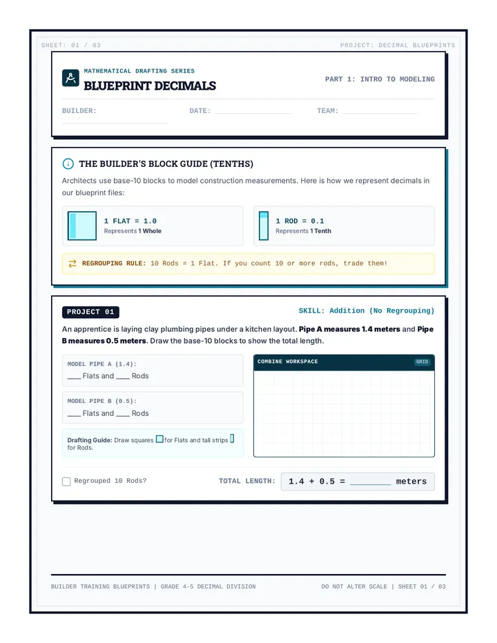
The Weather Paradox
In the city of Stochastopolis, tomorrow's weather depends only on today's weather.
• If it is Sunny today, there's an 80% chance it's Sunny tomorrow.
• If it is Rainy today, there's a 60% chance it's Rainy tomorrow.
Discussion
How can we draw this system?
What happens if it's Sunny today?
What is the chance of rain tomorrow?
THE MEMORYLESS PROPERTY
Markov Chain (Definition)
A stochastic process where the probability of the next state depends solely on the current state.
"The future is independent of the past, given the present."
// SYSTEM LOGIC
1
Discrete Time Steps ($t, t+1, t+2$)
2
Finite Number of States
3
Fixed Transition Probabilities
Anatomy of a Diagram
Schematic V1.0
S
Nodes (States)
Represent all possible conditions of the system.
Directed Edges
Arrows showing the movement between states over one time step.
0.85
Weights
The probability of that specific transition occurring.
RULE: The sum of probabilities leaving any node MUST equal 1.0 (100%).
GUIDED BUILD: COFFEE PREFERENCE
A customer either drinks Hot Coffee (H) or Iced Coffee (I) .
If they drink Hot today, there's a 70% chance they'll drink Hot tomorrow.
If they drink Iced today, there's an 80% chance they'll drink Iced tomorrow.
Diagram Area
H
I
Self-Loop (H → H): 0.70
Switch (H → I): ???
Self-Loop (I → I): 0.80
Switch (I → H): ???
Ready to Map?
You are now capable of taking complex behavioral patterns and turning them into mathematical circuits.
Identify
Label every possible state of the system.
Connect
Draw the arrows for every possible move.
Balance
Ensure outgoing edges sum to exactly 1.0.
State Scenarios Worksheet Schematic Worksheet: State Scenarios
Topic: Introduction to State Diagrams & Transitions
Unit: Markov Chains
ID: MC-L1-SYS
Student Name
Date
Class Period
1
System Definitions
1.1 In your own words, explain the "Memoryless Property" as it applies to a Markov Chain.
1.2 A system has two states: A and B. If the probability of staying in state A is 0.85, what must be the probability of transitioning from A to B? Explain why.
2
Mapping the Schematic
Scenario A: The Grocery Store. Shoppers at a boutique market either use the Self-Checkout (S) or the Attended Lane (A) . Historical data shows that if a shopper used Self-Checkout last time, there is a 90% chance they will use it again. If they used the Attended Lane last time, there is a 40% chance they will switch to Self-Checkout next time.
Construct the State Diagram below
Scenario B: Battery Life. An industrial drone has three battery states: High (H) , Medium (M) , and Low (L) .
From High: 60% stay High, 30% move to Medium, 10% move to Low.
From Medium: 50% stay Medium, 50% move to Low.
From Low: 100% of the time it is recharged and returns immediately to High.
Construct the State Diagram below
3
System Calibration
Below is a partial state diagram description. Calculate the missing values for the edges to ensure the system is stochastically valid.
Node X transitions:
X → Y 0.42
X → Z 0.18
X → X (Self-Loop) Answer: ________
Node Y transitions:
Y → X 0.55
Y → Y (Self-Loop) 0.25
Y → Z Answer: ________
4
Engineering a Model
Task: The Social Media Loop
Design a 3-state Markov model for an app user: Scrolling (S) , Posting (P) , and Offline (O) . Create your own realistic transition probabilities (ensure they sum to 1.0 for each state) and draw the resulting diagram.
Define your probabilities:
P(S→S): _____ P(S→P): _____ P(S→O): _____
P(P→S): _____ P(P→P): _____ P(P→O): _____
P(O→S): _____ P(O→P): _____ P(O→O): _____
State Diagram:
State Scenarios Answer Key ANSWER KEY: State Scenarios
Teacher Reference Only
Unit: Markov Chains
ID: MC-L1-KEY
1
System Definitions
1.1 Explain the "Memoryless Property".
Correct Answer: The memoryless property (or Markov property) states that the future state of a system depends only on the current state, and not on the sequence of events that preceded it. Mathematically: \(P(X_{t+1} | X_t, X_{t-1}, ..., X_0) = P(X_{t+1} | X_t)\).
1.2 P(A→A) = 0.85. What is P(A→B)?
Correct Answer: 0.15.
Reasoning: Because the system must transition to some state, the sum of all probabilities leaving a node must equal 1.0 (100%). \(1.0 - 0.85 = 0.15\).
2
Mapping the Schematic
Scenario A: The Grocery Store. S=Self, A=Attended.
Visual Representation Guide:
• Node S: Loop back to S with label 0.90 . Arrow to A with label 0.10 .
• Node A: Arrow to S with label 0.40 . Loop back to A with label 0.60 .
Scenario B: Battery Life. H, M, L.
Visual Representation Guide:
• Node H: Loop (0.60), to M (0.30), to L (0.10).
• Node M: Loop (0.50), to L (0.50). (No arrow back to H)
• Node L: Single arrow directly to H (1.00). (No self-loop)
3
System Calibration
Node X Answer:
0.40
Calculation: \(1.0 - (0.42 + 0.18) = 0.40\)
Node Y Answer:
0.20
Calculation: \(1.0 - (0.55 + 0.25) = 0.20\)
Matrix Blueprints Slides Module 02: Formal Systems
MATRIX BLUEPRINTS
Encoding Diagrams into Stochastic Matrices
The Translation Layer
State Diagram
A
B
Transition Matrix ($P$)
[ 0.8 0.2 ]
Why use Matrices?
Computers process arrays, not arrows.
Allows for heavy-duty algebra ($P^n$).
Standardizes multi-state systems.
THE TRANSITION MATRIX
TO STATE 1 TO STATE 2
FROM 1 FROM 2
[
\(P_{11}\)
\(P_{12}\)
\(P_{21}\)
\(P_{22}\)
]
Row Index = Where you are now.
Column Index = Where you are going.
Stochastic Rules
Rule #1
Every entry \(P_{ij}\) must be between 0 and 1.
\(0 \le P_{ij} \le 1\)
Rule #2
The sum of entries in each row must equal 1.
\(\sum_{j} P_{ij} = 1\)
"You must always end up somewhere."
The Build: 3-State Matrix
State Diagram
State A: 50% to A, 50% to B
State B: 20% to A, 70% to B, 10% to C
State C: 100% to A
[
0.5
0.5
0
???
???
???
1
0
0
]
Matrix Mastery
A transition matrix is just a state diagram in a more efficient suit.
Always check your rows. If they don't add to 1, your system is leaking probability.
P[i][j] = Probability(State_i → State_j)
Matrix Blueprints Worksheet Schematic Worksheet: Matrix Blueprints
Topic: Constructing Transition Matrices
Unit: Markov Chains
ID: MC-L2-BLUE
Student Name
Date
1
The Matrix Grid
Given the matrix \(P\) for a 3-state system (States 1, 2, 3):
\(P = \begin{bmatrix} 0.1 & 0.7 & 0.2 \\ 0.4 & 0.4 & 0.2 \\ 0.0 & 1.0 & 0.0 \end{bmatrix}\)
1.1 What is the probability of transitioning from State 1 to State 2?
1.2 Which state is "State 3" most likely to transition to next?
2
Drafting the Blueprint
Scenario: The Video Game AI
An AI character has three modes: Patrol (P) , Attack (A) , and Wait (W) .
• From Patrol: 70% chance to Patrol, 30% to Attack.
• From Attack: 40% chance to Patrol, 40% to Attack, 20% to Wait.
• From Wait: 100% chance to Patrol.
Construct the Transition Matrix P
[
]
3
Quality Assurance (Logic Testing)
Identify which of the following matrices are Stochastic Matrices . If they are not, explain why.
Matrix A:
\(\begin{bmatrix} 0.5 & 0.5 \\ 0.8 & 0.3 \end{bmatrix}\)
Valid Stochastic?
YES
NO
Reason: ___________________________
Matrix B:
\(\begin{bmatrix} 0.2 & 0.8 \\ 0.0 & 1.0 \end{bmatrix}\)
Valid Stochastic?
YES
NO
Reason: ___________________________
4
Engineering Challenge
The Smart Thermostat. A thermostat has three states: Heating (H), Cooling (C), and Off (O). The system never switches directly from Heating to Cooling (it must turn Off first). The chance of staying in Heating is 60%. The chance of staying Off is 80%. From Off, it is equally likely to turn to Heating or Cooling.
Create the transition matrix \(P\) for this system.
[
]
Matrix Blueprints Answer Key ANSWER KEY: Matrix Blueprints
Teacher Reference Only
Unit: Markov Chains
ID: MC-L2-KEY
1
The Matrix Grid
1.1 Probability from State 1 to State 2?
0.7 (Found at Row 1, Column 2)
1.2 Which state is State 3 most likely to transition to?
State 2 (Probability is 1.0)
2
Drafting the Blueprint
Correct Transition Matrix P (States: P, A, W)
[
0.7
0.3
0.0
0.4
0.4
0.2
1.0
0.0
0.0
]
Verification: Row 1 sum = 1.0 | Row 2 sum = 1.0 | Row 3 sum = 1.0
3
Quality Assurance
Matrix A:
NO
Reason: Row 2 sums to 1.1 (\(0.8 + 0.3 = 1.1\)). A stochastic matrix must sum to exactly 1.0 per row.
Matrix B:
YES
Reason: All entries are between 0 and 1, and all rows sum to exactly 1.0.
4
Engineering Challenge
Correct Transition Matrix P (H, C, O)
[
0.6
0.0
0.4
0.0
0.6
0.4
0.1
0.1
0.8
]
Note: If students choose different stay chances for Cooling, verify row sum = 1.0 and H→C = 0.
State Shifting Slides Module 03: Operational Logic
STATE SHIFTING
Predicting the Immediate Future
Where are we now?
The State Vector (\(v\))
A row vector representing the distribution of the system across all states at a specific time \(t\).
\(v^{(0)} = [ 0.4 0.6 ]\)
Example: 40% of customers are at Store A, 60% are at Store B.
Vector Properties
1 row, \(n\) columns.
Sum of all elements = 1.0.
Represents "System Status".
The Transformation Rule
\(v^{(1)} = v^{(0)} \cdot P\)
\(v^{(1)}\)
State at Time 1
\(v^{(0)}\)
Initial State
\(P\)
Transition Matrix
Calculating the Shift
[ x y ]
×
\(\begin{bmatrix} a & b \\ c & d \end{bmatrix}\)
=
[ (xa + yc) (xb + yd) ]
System Logic
To find the probability of being in State 1 tomorrow, we sum the probabilities of coming from every state to State 1.
1
Multiply Row by Column
2
Sum the Products
3
Result is a New Vector
Scenario: The Soda War
Market Status: Brand A has 70% share, Brand B has 30% share.
Customer Churn: Every month, 10% of A's customers switch to B. 20% of B's switch to A.
Step 1: Setup
\(v^{(0)} = [ 0.7 0.3 ]\)
\(P = \begin{bmatrix} 0.9 & 0.1 \\ 0.2 & 0.8 \end{bmatrix}\)
Step 2: Predict \(v^{(1)}\)
[ ??? ??? ]
Perform the multiplication now!
Outcome
\(v^{(1)} = [ 0.69 0.31 ]\)
After 1 month, Brand A dropped slightly to 69% and Brand B grew to 31%.
"The system has shifted."
State Shifting Worksheet Schematic Worksheet: State Shifting
Topic: Matrix Multiplication & Future Distributions
Unit: Markov Chains
ID: MC-L3-SHIFT
Student Name
Date
1
Status Assessment
1.1 Convert the following scenario into an initial state vector \(v^{(0)}\):
In a small town, 25% of the population owns an electric car, 60% own a gas car, and 15% own no car at all. Order the states as: [ Electric, Gas, None ].
[
]
2
The First Step
Problem 2.1: Binary System Calculation
Calculate \(v^{(1)} = v^{(0)} \cdot P\) given:
\(v^{(0)}\) [ 0.8 0.2 ]
\(P\) \(\begin{bmatrix} 0.9 & 0.1 \\ 0.3 & 0.7 \end{bmatrix}\)
Show Your Work:
Result \(v^{(1)}\):
Problem 2.2: The Trio Transition
[ 0.5 0.5 0.0 ]
\(\begin{bmatrix} 0.6 & 0.4 & 0.0 \\ 0.2 & 0.6 & 0.2 \\ 0.0 & 0.5 & 0.5 \end{bmatrix}\)
Result \(v^{(1)}\):
3
Case Study: Logistics Shift
The Delivery Drone Depot
A drone fleet is split between two bases: North (N) and South (S) . Currently, 100 drones are at North and 100 are at South.
Daily transition: 20% of North drones move South. 10% of South drones move North.
A) Write the Initial State Vector \(v^{(0)}\):
B) Write the Transition Matrix \(P\):
P = [ ]
C) Predict the drone distribution after 1 day (\(v^{(1)}\)):
Number of drones at North: ________ South: ________
State Shifting Answer Key ANSWER KEY: State Shifting
Teacher Reference Only
Unit: Markov Chains
ID: MC-L3-KEY
1
Status Assessment
1.1 Vector \(v^{(0)}\) [ Electric, Gas, None ]:
[
0.25
0.60
0.15
]
2
The First Step
Problem 2.1 Answer:
Calculation:
Col 1: \((0.8 \times 0.9) + (0.2 \times 0.3) = 0.72 + 0.06 = 0.78\)
Col 2: \((0.8 \times 0.1) + (0.2 \times 0.7) = 0.08 + 0.14 = 0.22\)
\(v^{(1)} = [ 0.78 0.22 ]\)
Problem 2.2 Answer:
Calculation:
Col 1: \((0.5 \times 0.6) + (0.5 \times 0.2) + (0 \times 0) = 0.3 + 0.1 = 0.4\)
Col 2: \((0.5 \times 0.4) + (0.5 \times 0.6) + (0 \times 0.5) = 0.2 + 0.3 = 0.5\)
Col 3: \((0.5 \times 0) + (0.5 \times 0.2) + (0 \times 0.5) = 0.1\)
\(v^{(1)} = [ 0.4 0.5 0.1 ]\)
3
Case Study Answers
A) Initial Vector \(v^{(0)}\):
[ 0.5 0.5 ]
(50% at each base)
B) Transition Matrix \(P\):
\(\begin{bmatrix} 0.8 & 0.2 \\ 0.1 & 0.9 \end{bmatrix}\)
C) Result after 1 day:
\(v^{(1)} = [ 0.45 0.55 ]\)
North: 90 drones | South: 110 drones
Calculation: 0.45 * 200 = 90; 0.55 * 200 = 110.
Time Leap Transitions Slides Module 04: Predictive Power
TIME LEAP TRANSITIONS
Forecasting Future States with \(P^n\)
One Step at a Time?
To predict the state after 3 steps (\(v^{(3)}\)), we could do this iteratively:
\(v^{(0)}\)
\(v^{(1)} = v^{(0)}P\)
\(v^{(2)} = v^{(1)}P\)
\(v^{(3)}\)
Is there a way to calculate \(v^{(3)}\) directly from \(v^{(0)}\)?
The Power of \(P\)
\(v^{(n)} = v^{(0)} \cdot P^n\)
To predict \(n\) steps into the future, raise the transition matrix
to the \(n\)-th power before multiplying by the initial state.
What is \(P^2\)?
\(P^2\) is the matrix where each entry \(P^2_{ij}\) represents the probability of starting in State \(i\) and ending in State \(j\) after exactly 2 steps.
Example: Rain/Sun
\(P^2 = P \cdot P\)
The Chapman-Kolmogorov Equation
The probability of moving from \(i\) to \(j\) in \(n\) steps is the sum of probabilities of all possible paths through any intermediate state \(k\).
\(P^{(m+n)} = P^m \cdot P^n\)
The Random Walker Challenge
A person walks between 2 rooms.
• If they are in Room 1, they have a 50% chance of staying and 50% chance of leaving.
• If they are in Room 2, they always leave and go to Room 1.
P Matrix
\(\begin{bmatrix} 0.5 & 0.5 \\ 1.0 & 0.0 \end{bmatrix}\)
Challenge
1. Calculate \(P^2\)
2. Calculate \(P^4\)
3. What do you notice about the rows as \(n\) increases?
Stability
In many Markov chains, as \(n \to \infty\), the rows of \(P^n\) begin to look identical.
This indicates a Steady State distribution where the system's probabilities stop changing.
"No matter where you start, you'll likely end up here."
Time Leap Transitions Worksheet Schematic Worksheet: Time Leap Transitions
Topic: n-Step Transitions & Matrix Powers
Unit: Markov Chains
ID: MC-L4-LEAP
Student Name
Date
1
Squaring the Transition
Given the transition matrix \(P\) for a 2-state system:
\(P = \begin{bmatrix} 0.8 & 0.2 \\ 0.5 & 0.5 \end{bmatrix}\)
→
Calculate \(P^2 = P \cdot P\)
[
]
Interpretation Check: Look at the top-left entry of your \(P^2\) matrix. What specific real-world probability does this value represent?
2
Two Steps Ahead
The Coffee Shop. Currently, 100% of customers drink Hot Coffee (\(v^{(0)} = [ 1.0 0.0 ]\)).
The transition matrix for 1 day is: \(P = \begin{bmatrix} 0.7 & 0.3 \\ 0.4 & 0.6 \end{bmatrix}\).
A) Use matrix multiplication to find the distribution after 2 days (\(v^{(2)}\)).
Formula Hint: \(v^{(2)} = v^{(0)} \cdot P^2\)
Result Vector \(v^{(2)}\):
3
The Equilibrium Shift
The matrix \(P^{10}\) for the Coffee Shop system is approximately: \(\begin{bmatrix} 0.57 & 0.43 \\ 0.57 & 0.43 \end{bmatrix}\).
3.1 If a customer starts by drinking Iced Coffee today, what is the probability they drink Hot Coffee 10 days from now?
3.2 What do you notice about the probability after 10 days, regardless of the starting beverage?
Critical Thinking: If you continue to raise P to higher powers (100, 1000, etc.), will the values change significantly? Why or why not?
Time Leap Transitions Answer Key ANSWER KEY: Time Leap Transitions
Teacher Reference Only
Unit: Markov Chains
ID: MC-L4-KEY
1
Squaring the Transition
Correct Matrix \(P^2\)
\(\begin{bmatrix} 0.74 & 0.26 \\ 0.65 & 0.35 \end{bmatrix}\)
Calculations:
R1C1: \((0.8 \times 0.8) + (0.2 \times 0.5) = 0.64 + 0.10 = 0.74\)
R1C2: \((0.8 \times 0.2) + (0.2 \times 0.5) = 0.16 + 0.10 = 0.26\)
R2C1: \((0.5 \times 0.8) + (0.5 \times 0.5) = 0.40 + 0.25 = 0.65\)
R2C2: \((0.5 \times 0.2) + (0.5 \times 0.5) = 0.10 + 0.25 = 0.35\)
Interpretation: The top-left entry (0.74) is the probability of starting in State 1 and being in State 1 exactly 2 time steps later.
2
Two Steps Ahead (Coffee Shop)
Step 1: Calculate \(P^2\)
\(\begin{bmatrix} 0.7 & 0.3 \\ 0.4 & 0.6 \end{bmatrix} \times \begin{bmatrix} 0.7 & 0.3 \\ 0.4 & 0.6 \end{bmatrix} = \begin{bmatrix} 0.61 & 0.39 \\ 0.52 & 0.48 \end{bmatrix}\)
Step 2: Calculate \(v^{(2)} = v^{(0)} \cdot P^2\)
\([ 1.0 0.0 ] \times \begin{bmatrix} 0.61 & 0.39 \\ 0.52 & 0.48 \end{bmatrix} = [ 0.61 0.39 ]\)
Answer: 61% Hot Coffee, 39% Iced Coffee after 2 days.
3
Equilibrium Answers
3.1 Start with Iced, Hot 10 days later?
0.57 (57%)
Found at Row 2, Column 1 of \(P^{10}\)
3.2 Observations?
Regardless of where you start (Row 1 or Row 2), the probability of being in State 1 is roughly the same (0.57). The initial condition matters less as time goes on.
Steady State Concept:
The system is converging to a fixed point where roughly 57% of customers drink Hot and 43% drink Iced. This is called the steady-state distribution (\(\pi\)). Further powers of \(P\) will eventually show no change in these values.
System Logic Lab Guide LAB REPORT: System Logic
Topic: Summative Markov Application Lab
Technical Ops
ID: MC-L5-LAB
Operational Brief: Fleet Optimization
The Velocity Rental Group manages a fleet of 1,000 cars across three locations: Airport (A) , Downtown (D) , and Suburbs (S) . As lead analyst, you must model the daily movement of cars to predict long-term demand and optimize parking capacity.
Movement Data (Daily Return Probabilities)
From Airport (A)
• 80% return to Airport
• 10% return to Downtown
• 10% return to Suburbs
From Downtown (D)
• 30% return to Airport
• 60% return to Downtown
• 10% return to Suburbs
From Suburbs (S)
• 20% return to Airport
• 10% return to Downtown
• 70% return to Suburbs
Objective Milestones
01
Schematic Design
Construct a complete state diagram showing all locations and transition probabilities.
02
Matrix Blueprint
Encode the diagram into a 3x3 stochastic transition matrix \(P\).
03
Operational Forecast
Given an initial distribution, calculate the fleet location after 1 day and 2 days.
04
Strategic Recommendation
Identify which location will eventually require the most parking space (long-term trend).
Begin Calculations
Proceed to the Response Sheet to record your technical analysis. Use a calculator for matrix powers. Ensure all vectors sum to exactly 1,000 cars in your final interpretation.
System Logic Lab Report Sheet Fleet Analyst Response Sheet
Lab: System Logic Optimization
Project: Velocity Rental
Lead Analyst
Date of Analysis
1
State Schematic Design
Map the three locations (A, D, S) and label all 9 possible transition edges with their respective probabilities.
2
Transition Matrix (P)
[
]
3
Inventory Forecast
Initial Status: On Day 0, the 1,000 cars are distributed as:
• 600 at Airport (A) | • 300 at Downtown (D) | • 100 at Suburbs (S)
Initial Vector \(v^{(0)}\):
A) Predict Distribution after 1 Day (\(v^{(1)}\)):
Cars at A: ______
Cars at D: ______
Cars at S: ______
B) Predict Distribution after 2 Days (\(v^{(2)}\)):
Cars at A: ______
Cars at D: ______
Cars at S: ______
4
Executive Summary
Based on your analysis, which location experiences the most "churn" (cars leaving) versus "retention" (cars staying)?
Strategic Parking Decision: Where should Velocity Rental Group build additional parking capacity for the long term? Justify using your calculations.
System Logic Lab Answer Key ANSWER KEY: System Logic Lab
Teacher Reference Only
Project: Velocity Rental
1 & 2
Schematic & Matrix Blueprint
Correct Transition Matrix P
\(\begin{bmatrix} 0.8 & 0.1 & 0.1 \\ 0.3 & 0.6 & 0.1 \\ 0.2 & 0.1 & 0.7 \end{bmatrix}\)
Diagram Check:
Node A: Loops 0.8, to D 0.1, to S 0.1.
Node D: Loops 0.6, to A 0.3, to S 0.1.
Node S: Loops 0.7, to A 0.2, to D 0.1.
3
Inventory Forecasts
Initial Vector \(v^{(0)}\):
[ 0.6 0.3 0.1 ]
Day 1 Distribution (\(v^{(1)}\)):
Calculation: \([0.6 \cdot 0.8 + 0.3 \cdot 0.3 + 0.1 \cdot 0.2, \dots]\)
\(v^{(1)} = [ 0.59 0.25 0.16 ]\)
Result: 590 Cars (A), 250 Cars (D), 160 Cars (S)
Day 2 Distribution (\(v^{(2)}\)):
\(v^{(2)} = [ 0.579 0.225 0.196 ]\)
Result: 579 Cars (A), 225 Cars (D), 196 Cars (S)
4
Executive Summary Answers
Churn vs. Retention:
The Airport (A) has the highest retention (80% stay). The Downtown (D) has the highest churn (40% leave, specifically 30% back to Airport).
Parking Decision:
Additional parking should be prioritized at the Airport (A) . Even though inventory drops slightly from 600, it remains the dominant location. However, a significant trend shows the Suburbs (S) growing rapidly (from 10% to nearly 20% in just two days). Long-term analysis (steady state) would show that the Airport will hold over 50% of the fleet consistently.